A Deep Dive into Voronoi Diagrams from the Ground Up
Introduction
Computing Voronoi diagrams is a fundamental problem in computational geometry with applications spanning robotics, computer graphics, spatial analysis, and beyond. While the naive \(O(n^2)\) algorithm is straightforward, Fortune's sweep line algorithm elegantly computes Voronoi diagrams in \(O(n \log n)\) time—optimal for the comparison model.
Fortune's algorithm isn't overly difficult conceptually, but anyone who ever attempted to implement it will be surprised by how scarce online resources are:
there do exist tutorials and toy demos online, but the vast majority of them cannot serve as reliable references. Many online demos omit essential components, and most tutorials stop at the same conceptual boundary without addressing the implementation details that make the algorithm genuinely challenging.
This project presents a complete and optimized implementation of Fortune's algorithm from the ground up, written in Crystal. It tackles all the non-trivial problems: numerical stability with degenerate cases, proper balanced tree operations, and complete DCEL (Doubly-Connected Edge List) construction. The project also includes a real-time visualizer built with SFML, show extra information about how the beach line and background data structure evolve in real time.
Real-time visualization of Fortune's algorithm in action. Watch the sweep line descend and the beach line evolve. As well as the Voronoi diagram emerging little by little.
What's Different
Many educational implementations simplify or omit certain details, which is understandable for teaching contexts but insufficient for a full, production-level understanding. This project aims to fill that gap:
Incomplete balancing: Many use simple BSTs without proper rebalancing, leading to \(O(n^2)\) worst-case behavior. Adding balancing is harder than just adding a plain AVL, since the beachline is not a traditional tree and has uncommon insertion rules (adding a new arc means splitting the original into two and inserting another. Depending on the implementation detail, this operation requires extra care.)
Degenerate cases not handled properly: Vertical line segments, co-circular points, and numerical precision issues are often ignored.
Oversimplified procedure and suboptimal data structures:
Fortune’s algorithm only reads like a clean sweep-line procedure on paper. In code,
the beach line's dual nature (spatial ordering + tree structure) requires careful design, and a lot of data structures also need to support uncommon operations.
Although performance is not a critical concern in a visualization, the underlying implementation should still reflect the actual algorithm. Presenting a faithful version ensures that the demo accurately represents what a production-level implementation must account for.
This implementation addresses all these issues with meticulous attention to detail, elegant code design, and comprehensive testing infrastructure
Why Implement Fortune's Algorithm?
Fortune's algorithm is famous in computational geometry, yet complete implementations are surprisingly rare.
Implementing it properly touches on multiple fundamental areas:
Algorithm design: Sweep line paradigm, event-driven simulation
Data structures: Balanced trees, priority queues, threaded pointers, half-edge meshes
Computational geometry: Parabola intersections, circle computations, planarity
Students who work through a complete implementation will be amazed by how beautifully these pieces fit together. It's a perfect example of how theoretical elegance meets practical engineering challenges. The algorithm is complex enough to be interesting, but structured enough that each component can be understood and tested independently.
This project aims to serve as a reference implementation that students can study, learn from, and use as a foundation for their own explorations in computational geometry.
Fortune's Algorithm: The Foundation
This article mainly serves to explain the project and also give some extra details omitted in most online demos, it assumes the readers have already tried following some tutorials online or attempted to implement the algorithm.
Besides discussions on the implementation details of the project itself, we won't talk too much about the basic ideas.
Here's a quick refresher on what Voronoi diagram is and how Fortune's algorithm works.
Problem Setup
The Voronoi diagram partitions the plane so that each region contains all points closest to a given site. Geometrically, every pair of sites defines a perpendicular bisector, and all Voronoi edges and vertices lie on these bisectors. This leads to an intuitive but expensive construction: for each site, intersect the half-planes that keep points closer to it than to others. Even with efficient half-plane intersection, doing this for all sites gives roughly O(n² log n) complexity, and more naive brute-force interpretations can degrade to O(n³). Fortune’s algorithm avoids enumerating all pairwise bisectors explicitly, achieving the optimal O(n log n) by maintaining a dynamic beach line and event structure instead.
Intuition
If we imagine knowing the Voronoi edges at a given sweep-line height y, then lowering the sweep line only perturbs their positions slightly; the combinatorial structure changes only at specific moments when two edges meet or an arc disappears. Fortune’s key insight is that these structural changes can be predicted and processed as discrete events, allowing the diagram to be built dynamically rather than recomputed from scratch at every step.
The parabola arises naturally from the distance definition: the set of points whose distance to a site equals their vertical distance to the sweep line forms a parabola with the site as its focus and the sweep line as its directrix. Each site therefore generates a parabolic arc on the beach line, and the intersection of two such parabolas marks points equidistant to both sites. When three parabolas intersect at a single point, that point is equidistant to all three corresponding sites, giving rise to a Voronoi vertex.
Because the distance to each site changes monotonically as the sweep line moves, the ordering of these parabolic arcs changes only at well-defined moments. These events—where one arc overtakes another or collapses—are exactly the times when the Voronoi structure changes. Fortune’s algorithm tracks these transitions explicitly, enabling an O(n log n) construction by reacting only to the discrete combinatorial updates rather than recomputing the geometry continuously.
The Sweep Line Paradigm
Fortune's algorithm uses a sweep line approach: imagine a horizontal line sweeping downward across the plane. At any moment, the sweep line is at height \(y = \ell\). The key insight is that we can determine which site "owns" any point above the sweep line by measuring distances in the metric induced by the sweep line.
The Beach Line
For a point \(p = (x, y)\) with \(y > \ell\) and a site \(s_i = (x_i, y_i)\) with \(y_i \geq \ell\), the "distance" from \(p\) to \(s_i\) is not the Euclidean distance, but rather the vertical distance from \(p\) to the parabola defined by focus \(s_i\) and directrix \(y = \ell\).
The parabola with focus \((x_i, y_i)\) and directrix \(y = \ell\) is given by:
The beach line is the lower envelope of all these parabolas—it consists of parabolic arcs, one for each site currently "active" above the sweep line.
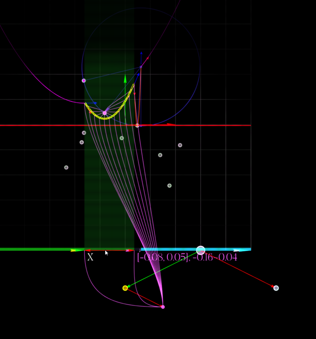
The beach line (highlighted in yellow) showing parabolic arcs. Each arc corresponds to a site, and breakpoints between arcs trace out Voronoi edges. The red horizontal line is the sweep line. The visualizer highlights the chosen arc, the region it occupies, and its tree node for further inspection.
Discrete Event Simulation
Fortune's algorithm is fundamentally a discrete event simulation. We initialize the event queue with all input sites (site events), sorted by y-coordinate. As we process events, new circle events may be discovered and added to the queue.
The Two Event Types
Site Events: When the sweep line reaches a new site \(s\), a new parabola is born. At the exact moment of contact, the parabola is degenerate—a vertical line segment at \(x = s_x\). This is because when \(y_i = \ell\), the denominator in our parabola equation becomes zero:
In the visualization, we always render the beach line with the sweep line slightly below the event point, so the arc already appears to have width. This is intentional—it helps visualize what's happening, but it's important to understand that at the exact event moment, it's a vertical segment.
In the beginning, we simply enqueue all the sites as events in the priority quene, then we proceed them one by one.
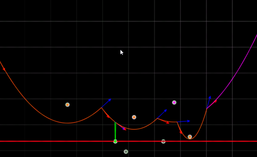
A new site event creating a degenerate arc (green vertical segment). In the visualization, the scanline is always intentionally moved down a bit, so that
the new arc isn't a vertical segment anymore. Blue arrows indicate derivatives at intersection points—these tell us which arc is above/below as we move left-to-right.
Circle Events: When three consecutive arcs \(A\), \(B\), \(C\) converge to a point, arc \(B\) disappears. This occurs when the sweep line reaches the bottom of the circumcircle through the three sites.
The key property: the beach line topology changes only at these discrete events. Between events, breakpoints move continuously but predictably—they trace out Voronoi edges.
Breakpoint Dynamics and Derivatives
A breakpoint between two arcs (corresponding to sites \(s_i\) and \(s_j\)) is the intersection of their parabolas. This breakpoint moves as the sweep line descends. The position \(x_b\) of a breakpoint satisfies:
As \(\ell\) decreases (sweep line moves down), \(x_b\) changes. Computing the derivative \(\frac{dx_b}{d\ell}\) tells us which direction the breakpoint moves. This is crucial for two reasons:
Arc ordering: At an intersection point, the derivatives of both parabolas tell us which arc is above/below as we move from left to right. If arc \(A\)'s parabola has a steeper positive slope than arc \(B\) at their intersection, then \(A\) is locally above \(B\) on the right side.
Circle event detection: We need to determine which arc gets squeezed into a point. By analyzing how breakpoints move, we can predict when three consecutive arcs will converge. The arc whose two surrounding breakpoints are moving toward each other is the one that will disappear.
Consider three consecutive arcs \(A\), \(B\), \(C\). Let \(x_{AB}\) be the breakpoint between \(A\) and \(B\), and \(x_{BC}\) between \(B\) and \(C\). If \(\frac{dx_{AB}}{d\ell} > 0\) (moving right) and \(\frac{dx_{BC}}{d\ell} < 0\) (moving left), and they're converging toward the same point, then \(B\) will be squeezed out — that's a circle event.
The Beach Line as a Balanced Tree
Why Trees Matter
The beach line stores arcs in left-to-right spatial order. We need to:
Find which arc is directly above a new site (during site events)
Insert new arcs when sites appear
Delete arcs when circle events occur
Query predecessor/successor arcs for circle event detection
All these operations need to be efficient: \(O(\log n)\) per operation. This demands a balanced binary search tree.
The Dual Nature: Spatial + Tree Structure
Most tutorials gloss over a critical design decision: where do we store the arcs? This question gets at the heart of what the beach line actually represents: it's both a spatial structure (arcs ordered left-to-right) and a search structure (we need fast queries).
Arc Ordering and Comparison
Before we discuss storage, we need to define what it means for arcs to be "ordered". Two arcs are adjacent in the beach line if their parabolas intersect, and we need to know which is on the left. This ordering is not based on site coordinates directly, but on the parabola geometry at the current sweep line position.
Finding the Arc Above a Point
When we say "find which arc is directly above a new site", we mean: if we shoot a vertical ray upward from the site, which arc does it hit first? This is the arc that will be split when the new site is inserted.
Naively, we could iterate through all arcs and check each one—but with \(n\) sites, that would be \(O(n)\) per query, giving \(O(n^2)\) total time. We need something faster.
The Search Tree Solution
Here's where the balanced search tree becomes essential. We can think of each parabola as defining a half-plane: the region where that site is closest. Since the tree stores arcs in sorted order based on their intersection points (the x-coordinates "where each arc extends out the most"), we can perform a binary search.
The key insight: if a parabola is completely covered by others, it's no longer in the tree. Only the arcs that are actually visible on the beach line (not dominated by other arcs) are stored. This means the tree size stays \(O(n)\) and queries are \(O(\log n)\).
Comparable Arcs
In the code, we define an Arc class that is comparable. Each time we compare two arcs, we do it based on their intersection point at the current sweep line position. This is a geometric computation: given two parabolas with foci at different sites and a shared directrix (the sweep line), we solve for their intersection.
Crucially, the shape of each parabola—and thus the intersection points—depends on where the sweep line currently is. As the sweep line descends, the parabolas change shape. This means arc comparison is dynamic and context-dependent.
Most implementations gloss over this: they assume you can just "compare" arcs, but the comparison is actually a sophisticated geometric computation. Getting this right, including handling edge cases where parabolas don't intersect or are degenerate, is essential for correct beach line maintenance.
Option 1: Arcs on Leaves Only
In this design, internal nodes represent breakpoints (intervals), and leaves represent arcs:
      [A|B]
     /      \
    A    [B|C]
        /     \
       B       C
Pros: Clean conceptual separation, breakpoints are explicit Cons: Internal nodes and leaves have different types, tree rotations become complex, harder to implement standard balanced tree algorithms
Option 2: Arcs on All Nodes (Our Choice)
In this design, every node stores an arc. The in-order traversal gives the left-to-right spatial ordering:
property value : Tproperty parent : BSTNode(T)?
In-order: A, B, C (left-to-right spatial order)
Pros:
Uniform node structure—every node is an arc
Standard balanced tree algorithms (AVL, Red-Black) apply directly
Rotations are clean and don't violate spatial ordering
Predecessor/successor queries are trivial (threaded tree pointers)
We chose Option 2. In-order traversal of a BST naturally gives the arcs in sorted order, and every tree node has the same data type. Less cases to handle.
Uncommon Data Structure Behaviors
Fortune's algorithm demands several data structures that behave in unusual ways. Understanding these quirks is essential for a correct implementation.
1. Balanced Tree with Non-Standard Insertion
Most balanced tree tutorials assume you insert one node at a time. But when a site event occurs in Fortune's algorithm, we need to:
Find the arc \(A\) above the new site
Split \(A\) into three nodes: \(A_{\text{left}}\), \(S_{\text{new}}\), \(A_{\text{right}}\)
Maintain the spatial ordering invariant during insertion
Rebalance the tree from the insertion point
This "triple insertion" violates the usual balanced tree contract. We can't insert the three nodes sequentially—intermediate states would break the in-order traversal property. Instead, we need a custom atomic insertion that handles all three nodes together, then triggers standard rebalancing.
2. Priority Queue with Random Access
The event queue is a priority queue sorted by y-coordinate. Standard priority queue operations are:
insert(event): Add a new event
pop_min(): Get the next event to process
Fortune's algorithm requires one capability that a standard binary heap does not provide: deletion of arbitrary events. When a circle event becomes invalid (because one of its arcs was replaced during another event), we must remove it from the event queue before it reaches the top.
This necessitates a priority queue that supports:
Handles or references to specific nodes in the heap
\(O(\log n)\) deletion by using those handles
Our implementation uses a custom priority queue where each event retains a direct pointer to its position inside the heap array. When an event becomes invalid, we delete it via its stored index and restore heap order in logarithmic time. This avoids the usual “lazy deletion” approach found in many educational implementations and ensures that the queue remains compact and accurate throughout the algorithm.
Among the various data-structure adaptations required by Fortune’s algorithm, this modification is the most straightforward.
3. Threaded Tree for \(O(1)\) Predecessor/Successor
To efficiently find predecessor/successor arcs, we use threaded pointers: each node maintains explicit pointers to its in-order predecessor and successor. This makes circle event checking \(O(1)\) after locating an arc.
Threading introduces overhead: every insertion and deletion must update not just the tree structure (parent/child pointers) but also the sequential links (prev/next pointers). This creates more places where bugs can hide—if the threads become inconsistent with the tree structure, you'll get incorrect results that are hard to debug.
However, the performance gain is absolutely worth it. In Fortune's algorithm, we need to check for potential circle events constantly. After inserting a new arc, we need to check if it forms a circle with its predecessor and successor. After a circle event, we need to check the newly-adjacent arcs. Without threading, finding a predecessor/successor requires tree traversal—\(O(\log n)\) in a balanced tree. With threading, it's \(O(1)\)—just follow a pointer.
Given that we perform these queries at least once per event, and there are \(O(n)\) events, threading saves us from \(O(n \log n)\) work down to \(O(n)\) for these queries. The added complexity is a price worth paying for this asymptotic improvement.
The Challenge of Unusual Data Structures
These data structure modifications—triple insertion, indexed priority queue deletion, and threading—are rarely covered in standard algorithms courses. Most tutorials gloss over them with "use a balanced tree" and "use a priority queue", leaving implementers to discover these issues through painful debugging.
Same-Site Arc Adjacency
Another subtle issue: multiple arcs can belong to the same site. When a new site splits an existing arc, the two resulting pieces both reference the original site. This means an arc's predecessor and successor in the beachline can reference the same site—requiring careful distinction between "same arc" vs "different arc, same site."
Operations that check arc identity (e.g., circle event validation) must compare arc pointers, not site references. When duplicating arc data for the split, we must decide what to copy vs share. These details are easy to get wrong and rarely discussed in textbooks.
This is a major reason why complete Fortune implementations are rare. The algorithm appears simple conceptually, but these data structure subtleties turn it into a significant engineering challenge.
The Tricky Parts
Degenerate Site Events
When a new site \(s\) appears, it creates a degenerate parabola (vertical line segment) at \(x = s_x\). This is the most numerically sensitive part of the algorithm.
The Initial Singularity
At the exact moment the sweep line touches \(s\), the parabola is degenerate:
The parabola equation becomes undefined. In practice, we handle this by recognizing that the new arc appears as an infinitesimally small segment, then immediately starts growing.
Splitting the Beach Line
When we insert a new site \(s\) into the beach line:
Find the arc \(A\) directly above \(s\) (query the tree at \(x = s_x\))
Split \(A\) into two arcs: \(A_{\text{left}}\) and \(A_{\text{right}}\)
Insert the new arc \(S\) between them
The challenge: Normal balanced trees assume you insert one node at a time. Here, we're inserting three nodes (two split pieces of \(A\) plus the new arc \(S\)) in a specific spatial configuration.
Maintaining Balance
We can't just insert three nodes sequentially—this would violate the spatial ordering invariant during intermediate states. Instead:
Create all three nodes: \(A_{\text{left}}\), \(S\), \(A_{\text{right}}\)
Set up their threaded pointers to maintain in-order invariant
Perform a custom "triple insert" operation that maintains tree balance
Update parent pointers and rebalance from the insertion point upward
In our AVL tree implementation, this requires careful height updates and potentially multiple rotations.
Circle Event Handling
Circle events are the most intricate part of Fortune's algorithm. Understanding why they're called "circle events" and how they predict Voronoi structure is crucial.
Why "Circle Event"?
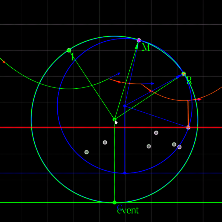
When we have three consecutive arcs on the beachline—corresponding to sites \(L\), \(M\), and \(R\) (left, middle, right)—their breakpoints trace out Voronoi edges. These two edges are the perpendicular bisectors between \(L\)-\(M\) and \(M\)-\(R\).
These two bisectors will eventually meet at a point that is equidistant from all three sites \(L\), \(M\), \(R\). This point is the center of the unique circle passing through all three sites—the circumcircle.
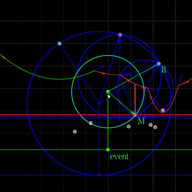
Circle Event Discovery: Three consecutive arcs (L, M, R) define a circle. When the sweep line reaches the bottom of this circle, the middle arc \(M\) will be squeezed to a point and disappear. The sites L, M, R are marked, and the circle passes through all three.
The key insight: when the sweep line reaches the bottom of this circle, all three sites are equidistant from that lowest point. At that moment:
The middle arc \(M\) disappears (squeezed to zero width)
Arcs \(L\) and \(R\) become adjacent
The center of the circle becomes a Voronoi vertex (where three edges meet)
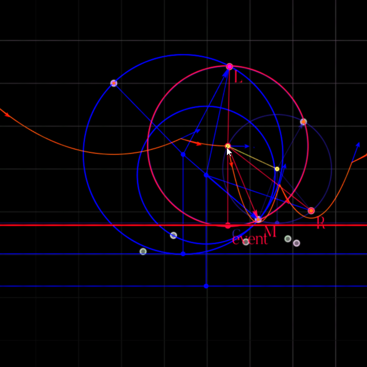
Circle Event Execution: As the sweep line reaches the bottom of the circle, the middle arc is squeezed to exactly zero width. The convergence point (circle center) becomes a Voronoi vertex where three edges meet. This is the moment the circle event triggers.
How to Detect Circle Events
Whenever we insert or remove an arc from the beachline, we check triplets of consecutive arcs. For each triplet \(L\), \(M\), \(R\):
Compute the circumcircle through sites \(L\), \(M\), \(R\)
Find the lowest point of the circle (center_y - radius)
Check if it's below the sweep line (future event)
Check if the breakpoints are converging (not diverging)
If all checks pass, add the circle event to the priority queue
The circumcircle center \((c_x, c_y)\) satisfies the system of equations:
This is solved using linear algebra. Nearly-collinear points lead to numerical instability, so we use robust geometric predicates with epsilon-tolerances to detect when points are too close to collinear.
Circle Event Invalidation: The Hidden Complexity
This is the detail most tutorials miss: Not all circle events actually trigger! When we detect a potential circle event (three consecutive arcs converging), we add it to the priority queue. But before it triggers, the beach line might change in a way that invalidates it.
Circle Event Invalidation: We were waiting for arc \(B\) to be squeezed by arcs \(A\) and \(C\). But then a different circle event causes \(C\) to be squeezed first! Now \(A\) and \(B\) are no longer adjacent to each other with \(C\) in between, so the original circle event (A-B-C) is invalid and must be skipped.
Consider the scenario illustrated above:
We detect that arcs \(A\), \(B\), \(C\) will converge → add circle event to queue
Before this event triggers, arc \(C\) gets squeezed by other arcs
Now \(A\) and \(B\) are no longer adjacent in the beachline
The circle event (A-B-C) is now invalid and should be discarded
Implementation approach: Each circle event stores pointers to the three arcs involved. When the event pops from the priority queue, we check:
Are these three arcs still consecutive in the beachline?
Are they in the same left-to-right order?
Have any of them been deleted?
If any check fails, we discard the event and continue. This lazy invalidation strategy is simpler than trying to remove invalidated events from the priority queue. The cost is minimal—we just skip stale events when we pop them.
Why This Matters
Getting circle event invalidation wrong leads to:
Crashes: Accessing deleted arc pointers
Incorrect output: Spurious Voronoi vertices at wrong locations
Topology errors: DCEL becomes inconsistent
This is where most bugs in Fortune implementations come from. The algorithm looks simple on paper, but correctly handling event invalidation requires careful pointer management and validity checking. This is a detail that's easy to overlook but catastrophic to get wrong.
Implementation Highlights
Direction Abstraction for Symmetric Operations
Most balanced tree implementations duplicate code for left and right operations. Our approach uses direction abstraction to achieve complete symmetry, eliminating code duplication and an entire class of mirror-image bugs.
The Direction Enum
Instead of writing separate rotate_left and rotate_right functions, we define:
enumDirectionLeftRightdefopposite : Directionself == Left ? Right : Leftendend
Unified Rotation
A single rotation function handles both directions:
Now rotate_left and rotate_right are just thin wrappers:
defrotate_left
rotate(Direction::Left)
enddefrotate_right
rotate(Direction::Right)
end
Double Rotations Through Composition
AVL trees sometimes require double rotations (LR and RL cases). With our symmetric design, these become trivial compositions:
defdouble_rotate(dir : Direction) : BSTNode# First rotate the child in the opposite direction
child_node = child(dir.opposite)
set_child(dir.opposite, child_node.rotate(dir.opposite))
# Then rotate self in the primary direction
rotate(dir)
end
This single function handles all double rotation cases. The LR rotation (Left-Right) is double_rotate(Direction::Left), and the RL rotation (Right-Left) is double_rotate(Direction::Right). No code duplication, no asymmetry, no room for subtle bugs where one case is handled differently from its mirror.
The beauty of this approach: we write the rotation logic once, prove it correct once, and it automatically works for all cases. This is not just aesthetically pleasing—it eliminates an entire class of bugs where left/right cases diverge.
Visual Debugging Infrastructure
Implementing complex algorithms like Fortune's requires rigorous validation. We can't just run the code and hope it works—with geometric algorithms, subtle bugs can hide in edge cases that only appear with specific input configurations.
To ensure 100% correctness, I built a comprehensive visual debugging system. The test suite doesn't just check that operations complete—it generates interactive HTML reports showing every single step of execution.
Tree structure before and after each operation (insert, delete, rotate)
Highlighted nodes involved in rotations and rebalancing
Height/color annotations to verify balance properties
Operation sequence with detailed explanations
Visual diff showing exactly what changed
This infrastructure was absolutely essential. When a test fails, I don't just get a boolean "failed"—I get a complete visual history showing exactly where the tree structure diverged from expected. This turned debugging from guesswork into systematic analysis.
Building this debugging infrastructure took almost as long as implementing the algorithms themselves. But it's a perfect example of the engineering philosophy behind this project: if you're going to build something complex, build the tools to validate it. The confidence that comes from knowing every edge case is tested and visualized is worth the investment.
Numerical Robustness
Numerical precision is one of the most challenging aspects of implementing Fortune's algorithm. The naive approach leads to catastrophic failures in edge cases.
Degenerate Arc Initialization
When a new site appears, its "parabola" at the exact moment the sweep line touches it is degenerate—mathematically undefined. The parabola equation \(y = s_y + \frac{(x - s_x)^2}{2(s_y - \ell)}\) has a division by zero when \(s_y = \ell\).
The key insight: at this singularity, the parabola degenerates into a vertical ray pointing upward from the site. We handle this by:
Treating new arcs as rays initially: Don't immediately compute parabola intersections
Using limit behavior: As \(\ell \to s_y^-\), the parabola becomes increasingly steep, approaching a vertical line
Deferring intersection computation: Only compute breakpoints after the sweep line has descended past the site
In the code, we implement this by checking if the arc is "active" (sweep line has moved past its site) before computing intersections. This is theoretically correct: at the limit case, the new arc occupies zero width and immediately splits an existing arc.
Parabola Intersection Edge Cases
Computing the intersection of two parabolas requires solving a quadratic equation. The implementation in arc.cr handles several edge cases:
# Solve: a*x² + b*x + c = 0
a = d1 - d2
b = 2*(x2*d2 - x1*d1)
c = (x1**2 + y1**2 - directrix**2)*d1 - (x2**2 + y2**2 - directrix**2)*d2
delta = b**2 - 4*a*c
return [] ofPointif delta < 0# No intersectionif delta == 0# Tangent (rare but possible)
xx0 = (-b)/2.0/a
return [Point.new(xx0, eval_at(xx0))]
end# Two intersections - use both
xx1, xx2 = (-b - Math.sqrt(delta))/2.0/a, (-b + Math.sqrt(delta))/2.0/a
return [Point.new(xx1, eval_at(xx1)), Point.new(xx2, eval_at(xx2))]
Other Degenerate Cases
Vertical site events: Sites with identical x-coordinates create parallel parabolas (no intersection)
Co-circular points: Four or more sites on the same circle create degenerate circle events
Collinear sites: Sites forming a line produce infinite Voronoi edges that must be clipped to the bounding box
Duplicate sites: Multiple sites at the same location are filtered during preprocessing
Rather than using rational arithmetic (which would be slow), we use careful floating-point handling with geometric predicates that check for degenerate configurations before performing problematic computations. This is much faster than symbolic math while maintaining correctness.
DCEL Construction
The output of Fortune's algorithm is a Doubly-Connected Edge List (DCEL), a standard data structure for representing planar subdivisions that enables efficient traversal and queries.
Half-Edge Basics
A DCEL represents edges as pairs of directed half-edges. Each half-edge stores:
Origin vertex: The vertex it starts from
Twin: The oppositely-directed half-edge on the same geometric edge
Next/Prev: Pointers to adjacent half-edges around the incident face
Incident face: The Voronoi cell this half-edge bounds
This structure allows \(O(1)\) navigation: given a half-edge, you can instantly find its origin, destination (twin.origin), the face it bounds, and walk around that face.
Incremental Construction During Fortune's Algorithm
The tricky part: DCEL edges are constructed incrementally as the sweep line descends. This creates several challenges:
Ray-to-Segment Transition
When a new arc appears (site event) or an arc disappears (circle event), we create a new Voronoi edge. Initially, this edge has:
One known vertex: The circle event point (if any)
Unknown endpoint: The other vertex will be determined by a future event
We represent this as a half-edge with null destination. The implementation tracks these "open" half-edges:
Halfedge
@orig : Site | Nil# Known start vertex
@dest : Site | Nil# Initially nil, filled later
@twin : Halfedge | Nil
@incident_face : Face | Nil
As the algorithm progresses:
First vertex added: Edge exists as a ray with known origin, unknown destination
Second vertex added: Edge becomes fully determined, both orig and dest are set
Some edges never close: Infinite rays extending to the bounding box remain open until post-processing
Stitching the Mesh
During circle events, we must connect half-edges to form complete face boundaries. This requires:
Maintaining arc-to-edge mappings: Each arc tracks its left and right bounding edges
Updating twins: When edges are created, ensure twin pointers are set correctly
Linking next/prev: Close the face boundary by connecting half-edges in counter-clockwise order
The final result is a complete topological structure where every face is a valid Voronoi cell, every edge has a twin, and you can traverse the entire diagram efficiently. This enables downstream applications like nearest-neighbor queries, interpolation, and path planning.
GL-Powered Visualizer using SFML
The real-time visualizer is built using CrSFML (Crystal bindings to SFML - Simple and Fast Multimedia Library). Rather than using a high-level UI framework, we built a custom rendering system from scratch, giving complete control over visual appearance and performance.
Custom Graphics Pipeline
The visualizer renders complex geometric primitives in real-time:
Smooth animations: Sweep line descends with easing functions for visual clarity
Real-time parabola rendering: Hundreds of curved arcs per frame, computed on-the-fly
Dynamic highlighting: Arcs and breakpoints change color during events
Tree structure overlay: Live visualization of the AVL tree structure for debugging
Event queue display: Shows upcoming site and circle events with color coding
OpenGL-Accelerated Rendering
SFML provides OpenGL-accelerated rendering, which is essential for smooth animation. Each frame, we:
Compute parabola curves: Evaluate each arc's equation at multiple points
Tessellate into line segments: Convert curves to polylines for GPU rendering
Batch draw calls: Minimize state changes for performance
Update overlays: Redraw UI elements (text, buttons, status indicators)
All rendering is done from scratch using SFML's low-level primitives. No external UI libraries—just direct vertex manipulation and shader-free 2D graphics. This gives us the flexibility to implement custom visual effects while maintaining 60+ FPS even with complex diagrams.
Crystal: The Language Choice
Why Crystal?
I've written code in many languages over the years,
but Ruby holds a special place.
Its expressiveness, and its ability to make code read like prose are unmatched.
But Ruby has one major drawback: performance. For a computationally intensive algorithm like Fortune's, where we're manipulating complex data structures and performing geometric computations thousands of times per second, the interpreted nature of Ruby becomes a bottleneck.
Enter Crystal: a language that captures Ruby's elegance while compiling to native code. Crystal's syntax is intentionally Ruby-like, and many Ruby programs run in Crystal with minimal changes. But under the hood, it's statically typed and compiled via LLVM, giving you C++-level performance.
Crystal offers:
Performance: Native code compilation, no garbage collection pauses during tight loops
Type safety: Static type checking catches errors at compile time, but with inference so you don't sacrifice readability
Expressiveness: Ruby's elegance—blocks, iterators, method chaining—without the runtime penalty
Generics: Powerful type parameters with compile-time specialization
For me, Crystal hits the sweet spot: I can write beautiful, expressive code that feels like Ruby, but get the performance needed for serious computational geometry. It's the best of both worlds.
Partial Specialization
Crystal's generics are specialized at compile time. The compiler generates optimized code for each concrete type:
class AVLTree(T)
  def insert(value : T)
    # Specialized for Int32, Float64, String, etc.
  end
end

tree_int = AVLTree(Int32).new
tree_str = AVLTree(String).new
This gives us zero-cost abstractions—generic code with C++ template-like performance.
Union Types
Crystal's union types handle nullable pointers elegantly:
property left : AVLNode(T) | Nil

if left_child = @left
  # left_child is guaranteed non-nil here
  left_child.do_something
end
Ruby Compatibility
Crystal's syntax is intentionally close to Ruby, making it approachable:
# Ruby-like syntax
sites = [Point.new(1, 2), Point.new(3, 4)]
sites.each { |s| puts s }

# But with compile-time type safety!