Background

Welcome! This project develops a flexible simulation framework for continuous-wave (CW) time-of-flight (TOF) imaging and uses it to investigate how CW-TOF measurements can be repurposed to achieve single-shot depth estimation through a mechanism analogous to off-axis holography.

Off-Axis Holography and CW Time-of-Flight Sensing

Off-axis holography and continuous-wave (CW) time-of-flight (TOF) sensing represent two distinct but mathematically related approaches to recovering scene information from modulated optical signals.

Off-axis holography uses a tilted reference wave to heterodyne the object field in space. The interference pattern contains a shifted cross-term that can be isolated in the Fourier domain, enabling single-shot recovery of the complex optical field (amplitude and phase). This requires spatial filtering but no temporal modulation.

CW-TOF sensing, in contrast, relies on temporal modulation. A modulated illumination signal is reflected by the scene and correlated with a reference waveform inside the sensor through lock-in demodulation. By sampling multiple phase shifts, the system estimates the propagation delay and recovers per-pixel distance.

Although framed differently, both techniques rely on heterodyning and correlation, implemented either optically in space or electronically in time.

We propose a new method that takes advantage of off-axis holography and show that with specific setup of the sensor and light source, the depth of the scene can be reconstructed from one single image. We show the theoretical derication, reasoning on the detailed setups, and the results produced by our implementation.

From an implementation standpoint, the system is fundamentally a CW-TOF pipeline: light sources emit temporally modulated signals, and the sensor performs lock-in correlation with a reference waveform. The core objective is not to replicate off-axis holography directly, but to show that a properly configured CW-TOF system can reproduce off-axis behavior — and thus recover complex-valued scene information from a single exposure.

Implementation-wise, the system is an entirely CW-TOF pipeline with extra options: light sources emit temporally modulated signals, and the sensor performs lock-in correlation with the reference waveform. The path tracer is extended to support time-resolved propagation, modulated emitters of various types, and modulated sensors capable of gated or heterodyne measurements. This creates a general-purpose environment in which a wide range of spatiotemporal modulation schemes can be tested.

The renderer is built around a time-resolved path tracer with support for a wide set of interchangeable modules, including:

Modulated Light sources: arbitrary waveform generators, point and line laser scanners
Modulated Sensors: global-shutter and rolling-shutter detectors
Auxiliary Controls: configurable per-pixel synchronization between the light source and sensor activation

This modular design enables us to explore a large family of spatiotemporal modulation schemes, many of which cannot be tested easily in real hardware.

Theory-wise , the core contribution is deriving the conditions under which a CW-TOF sensor, combined with spatial heterodyning, produces an isolatable cross-correlation term—equivalent to the off-axis holography cross-term—and can therefore recover a complex field from a single shot. The analysis also reveals that several configurations that appear valid at first glance actually fail due to subtle issues such as spatial–temporal aliasing, mismatch between the heterodyne carrier and the sampling lattice, or destructive mixing of undesired interference terms.

Using the modular simulation framework, we validate these insights experimentally. Configurations predicted to succeed do indeed produce clean reconstructions, while the ones predicted to fail exhibit exactly the artifacts anticipated by the theory. The simulator thus serves both as an engineering platform for modulated light transport and as a tool for understanding the delicate conditions under which spatial and temporal heterodyning interact.

For demonstration, we perform all the tests in this simple Cornell Box scene (with the light source removed). For some tests, we also changed some materials in the scene to make some unwanted artifacts stand out more.

Basic Setup & Derivation

Core idea: When a modulated light signal travels through the scene and reflects off surfaces, the returned waveform carries a measurable delay. Correlating this signal with the known modulation pattern enables recovery of the distance to each point in the scene.

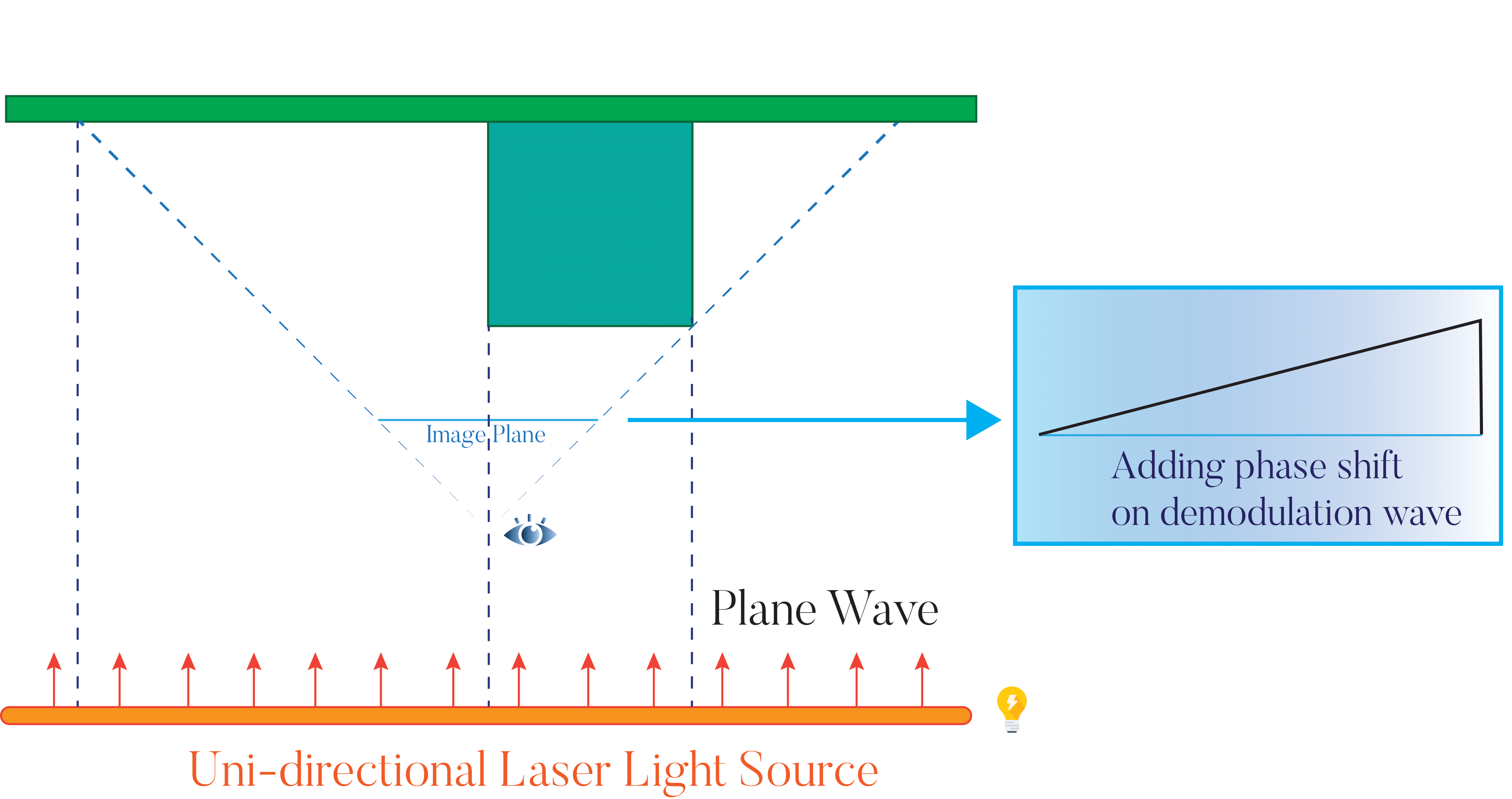
Assume we have such a setup: the original carrier wave $E_c$ gets sent out and returns after hitting the scene, creating the object wave $E_o$. The reference wave $E_r$ is used to control the sensitivity of the sensor for demodulation.

If we send out a plane wave, then each position has the same phase in the carrier wave:

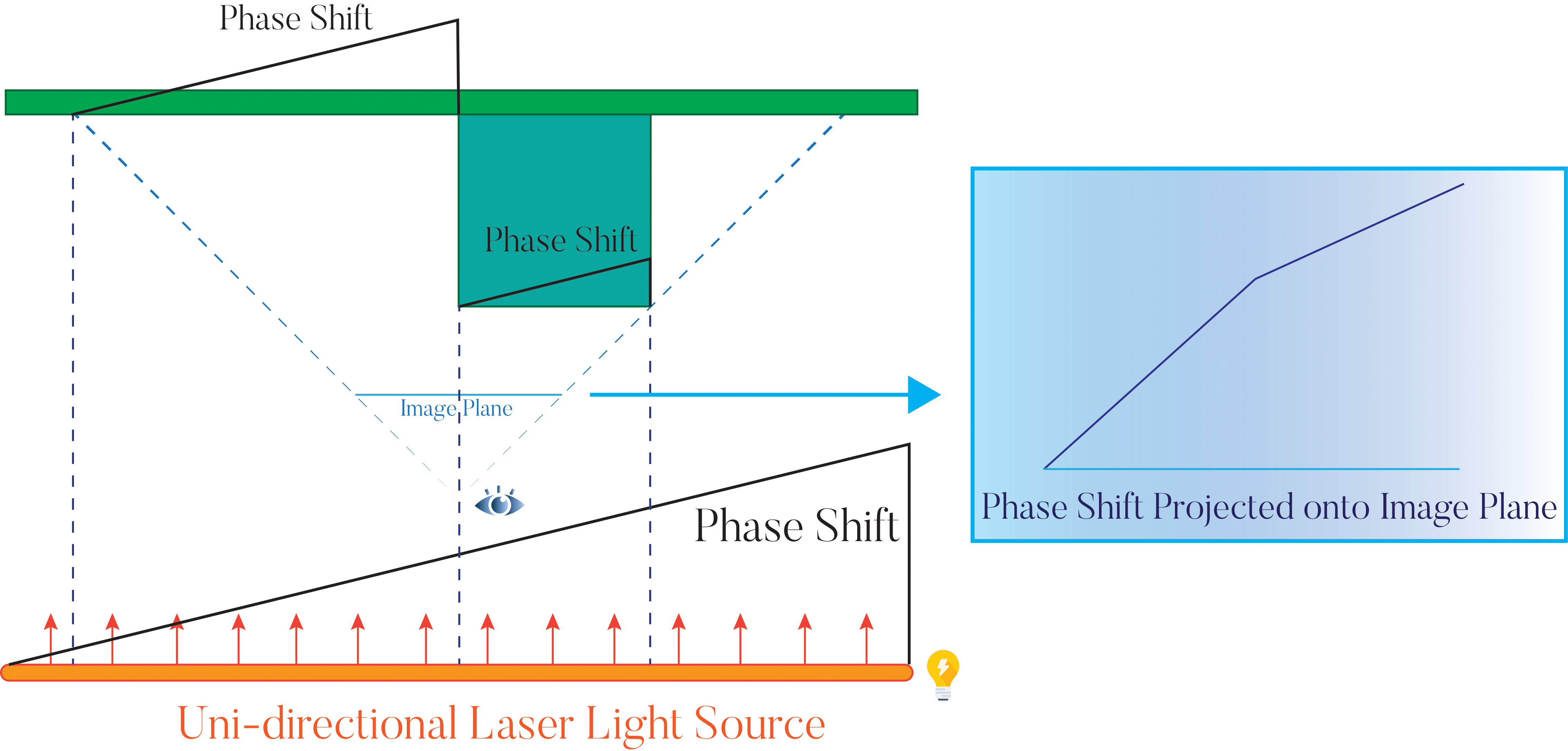
\[\begin{align} \text{Carrier wave:~}&E_c = \cos(\omega t) \\ &\text{the original wave to send out} \\ \text{Object wave:~}&E_o = A \cos(\omega t - \phi(x,y)) \\ &\text{phase delay $\phi$ depends on the position $(x,y)$} \end{align}\]

In a normal off-axis holography camera, a tilted plane wave is used to interfere with the object wave. Here, if the sensor supports a rolling-shutter-like functionality that allows different pixels to have a differently phase-shifted demodulation wave, we can do something similar by using a tilted plane wave for demodulation, for example, we add a phase shift that's proportional to x position:

\[\begin{align} \text{Reference wave:~} &E_r = \cos(\omega t + \kappa \cdot x) \end{align}\]

Now we take the cross-correlation between $E_r$ and $E_o$:

\[\begin{align} I(x,y) &= \lim_{T\rightarrow\infty} \int_{-\frac{T}{2}}^{+\frac{T}{2}} \frac{A}{T} \cos(\omega t + \kappa \cdot x)\cos(\omega t - \phi(x,y)) \mathrm{d}t \\ &= \frac{A}{2} \cos(\kappa \cdot x + \phi(x,y)) \end{align}\]

If we take the Fourier transformation:

\[\begin{align} F[I](k_x,k_y) &= \int_{-\infty}^\infty \int_{-\infty}^\infty \frac{A}{2} \cos(\kappa \cdot x +\phi(x,y)) e^{-2\pi j(k_x x + k_y y)} \mathrm{d}x\mathrm{d}y \\ &= \frac{A}{4} \iint e^{ j(\kappa\cdot x + \phi(x,y)) -2\pi j (k_x x + k_y y)} + e^{ -j(\kappa\cdot x + \phi(x,y)) -2\pi j(k_x x + k_y y)} \mathrm{d}x\mathrm{d}y \end{align}\]

This has 2 components, we call them $g_1$ and $g_2$:

\[\begin{align} g_1 &= \frac{A}{4} \iint e^{ j(\kappa\cdot x + \phi(x,y)) -2\pi j (k_x x + k_y y)} \mathrm{d}x\mathrm{d}y \\ g_2 &= \frac{A}{4} \iint e^{ -j(\kappa\cdot x + \phi(x,y)) -2\pi j (k_x x + k_y y)} \mathrm{d}x\mathrm{d}y \end{align}\]

Since:

\[\begin{align} g_1 &= \frac{A}{4} \iint e^{ j(\kappa\cdot x + \phi(x,y)) -2\pi j (k_x x + k_y y)} \mathrm{d}x\mathrm{d}y \\ &= \frac{A}{4} \iint e^{ j \phi(x,y) -2\pi j (k_x x + k_y y)} e^{j(\kappa\cdot x) } \mathrm{d}x\mathrm{d}y \\ &= \frac{A}{4} F[e^{ j \phi(x,y)}](k_x - \kappa, k_y) \end{align}\]

Similarly:

\[\begin{align} g_2 = \frac{A}{4} F[e^{ -j \phi(x,y)}](k_x + \kappa, k_y) \end{align}\]

As we can see, from this setup, we expect to see 2 images centered at $[\kappa,0]$ and $[-\kappa,0]$. We can use either of them to reconstruct a hologram that includes the phase $\phi$ (first shifting it back to the center, then take the inverse Fourier transformation).

As long as we can create a phase shift that only linearly depends on the spatial pixel position on the image, this will work, or else it's not simply a translation anymore. We'll give more details in the next section.

Observations and Caveats

The setup described above only works under very specific conditions, and not merely because of parameter tuning. There are multiple ways to introduce the carrier and reference waves—through illumination delay, sensor-side tilts, or reference-phase shifts—but only a subset of these configurations produces a usable cross-term. Certain classes of configurations are fundamentally incapable of producing an isolatable cross-term, regardless of how their parameters are adjusted. These failures arise from structural incompatibilities in how spatial and temporal heterodyning interact with the sensor’s sampling process.

One thing we can notice is that: adding a phase shift on the object wave will have the same effect as adding one to the demodulation wave. Instead of:

\[\begin{align} \text{Carrier wave:~}&E_c = \cos(\omega t) \\ \text{Object wave:~}&E_o = A \cos(\omega t - \phi(x,y)) \\ \text{Reference wave:~} &E_r = \cos(\omega t + \kappa \cdot x) \end{align}\]

we can also do:

\[\begin{align} \text{Carrier wave:~}&E_c = \cos(\omega t - \kappa \cdot x) \\ \text{Object wave:~}&E_o = A \cos(\omega t - \kappa \cdot x - \phi(x,y)) \\ \text{Reference wave:~} &E_r = \cos(\omega t) \end{align}\]

The important thing is that either way we do it, the extra phase shift $\kappa \cdot x$ has to be linear with respect to pixel position $x$. Since the phase shift rate $\kappa$ directly determines the amount of shift in the frequency domain, if it's not constant across the whole image, that means different frequency component gets shifted differently and there's not a single central frequency shift anymore.

Some seemingly correct setup will fail due to this.

An example of a setup that doesn't work. It's easy to visually tell that the stripes have different widths.

The setups that won't work

Sweeping a thin laser source and use an un-tilted plane wave for demodulation.
Using a quad laser light on which different positions activates with a delay depending on the position and an un-tilted plane wave for demodulation.
Using a tilted quad laser light and an un-tilted plane wave for demodulation.

As we can see, the left and right halves of the image plane correspond to different amounts of phase shift, causing $\kappa$ to be varying across the whole image.

These are basically the same. They all create a tilted plane wave as the carrier wave. The main issue with this type of setup is that the phase shift depends on the position on the light source not the position on the image. The position on the light source directly corresponds to the position of the hitpoint in the scene, and this will cause the phase shift/pixel position rate to differ depending on how far the object is. As a result, in the frequency domain, different parts of the scene will be shifted differently and there won't be a central frequency, meaning we can't expect to shift it to the center and demodulate using one single frequency.

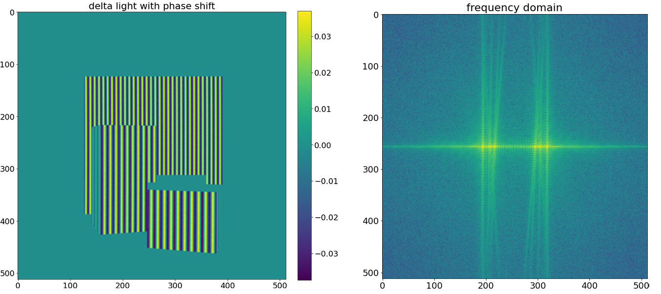
An example of a setup that doesn't work. As we can see, the 3 streaks correspond to the 3 regions with different pattern widths.

If there're multiple objects at multiple distances, they will be shifted differently in the frequency domain; the same happens if there's one big object with a ramp. If we can first separate the frequency components, this kind of setup could potentially work, but it requires extra work.

The one on the left (shifted quad light) doesn't work, and the one on the right (shifted demodulation wave) works. As we can tell visually, in the image produced by a non-working setup, the stripes have different width on different regions, corresponding to a different frequency component. We can't make 2 frequency components centered at the same time with one single phase shift.

For this type of setup to work directly, we need an orthographic camera, so that now $\kappa$ doesn't depend on the depth anymore and is constant. Besides using an orthographic camera, there're other easier working setups:

The setups that can work

If we can modulate pixels differently, we can simply make the demodulation wave tilted instead, as discussed above:

A plane wave as the carrier wave and a tilted plane wave for demodulation.

An example of a working setup, as we can see, one key difference is that the width of the stripes doesn't depend on the distance anymore. Since it's still a unidirectional light, the side walls are completely invisible.

A plane wave as carrier and tilted plane wave as demodulation wave. In this setup, the walls are completely dark since they're parallel to any light emitted from the light source, making them contain no depth information. The lit parts are reconstructed properly.

In fact, the carrier wave can be anything, as long as we can have a tilted plane wave for demodulation.

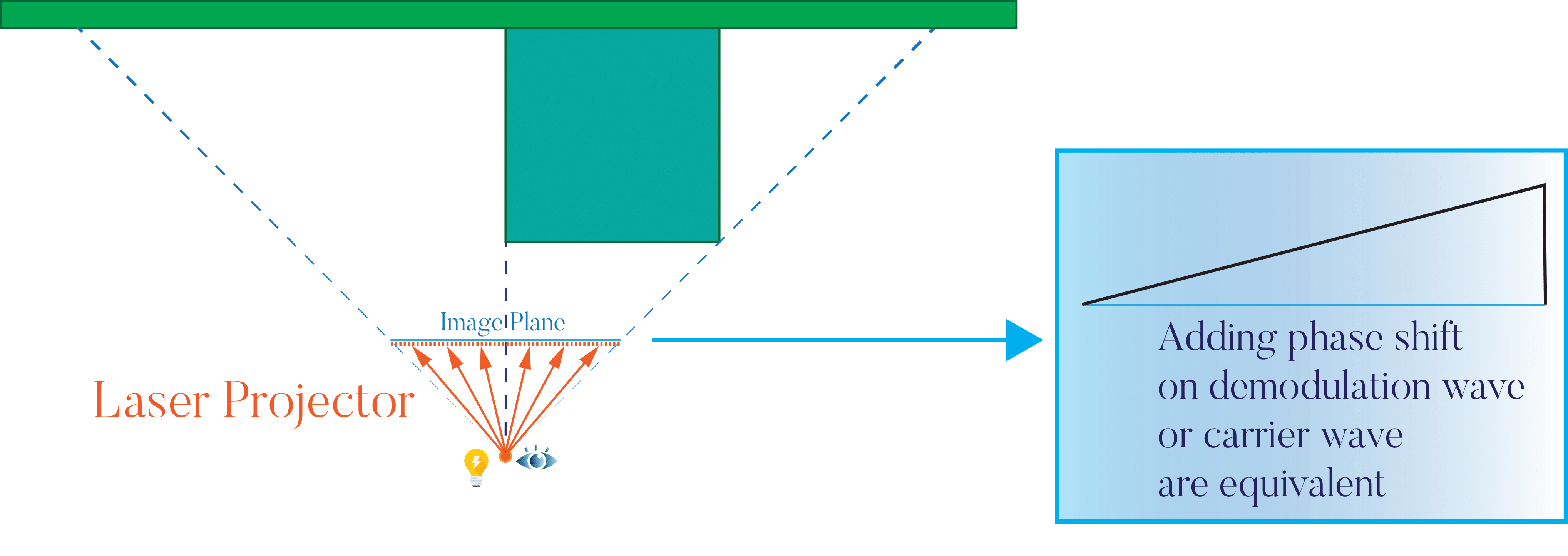
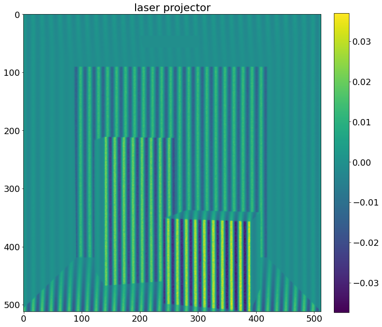
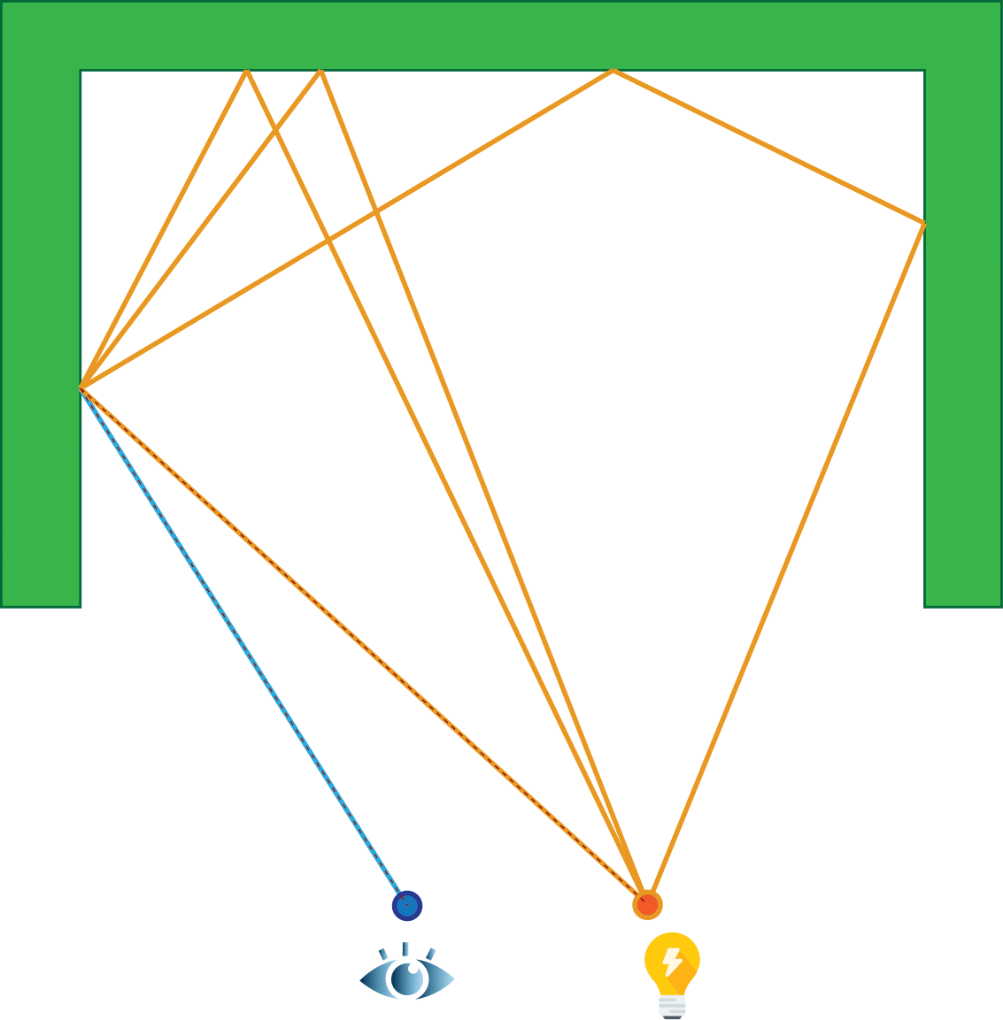
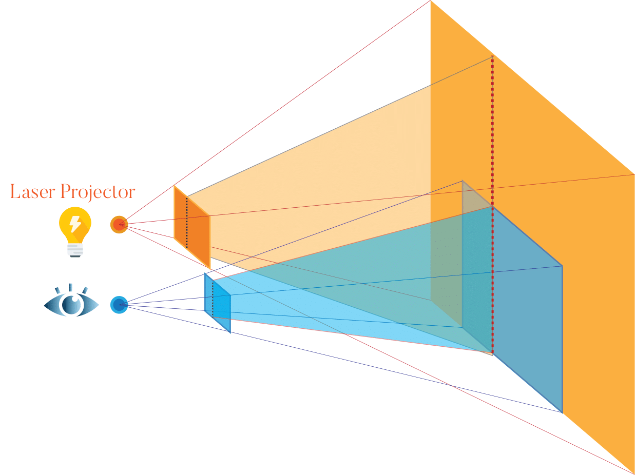
A laser projector as the light source and a tilted plane wave for demodulation.

With a laser projector, another option is to add the phase shift on the carrier wave, since it's possible to make the phase shift $\kappa \cdot x$ if we set it up properly:

A laser projector with phase shift depending on the pixel position as the light source and an un-tilted plane wave for demodulation.

This is easy to implement by using a rotating mirror to reflect a line source, as done in some other papers.

With a laser projector, we can generate the exact same result adding a phase shift on either the light source or the demodulation wave.

With a laser projector, the most noticeable visual difference is that now all the side walls are illuminated, as expected. Adding the phase shift on the light source or the sensor are equivalent and can produce the exact same results when tuned properly.

The depth reconstructed using the laser projector setup. This one also includes the side walls.

Indirect Lighting

In practical environments, light rarely follows a single line-of-sight path. Instead, it undergoes multiple reflections, refractions, and scattering interactions, which introduce higher-order light transport terms that substantially complicate the measurement process.

The previous section focused on direct lighting, but in reality, we expect the light to bounce in the scene multiple times, making the problem more challenging.

Each pixel corresponds to one camera ray hitting one position in the scene. With a laser source, we expect each shaded point in the scene to correspond to one single ray. As a result, each pixel only corresponds to one single path and one single distance.

Single scatter: each shading point only corresponds to one light path.

For multi-scatter, this is not the case anymore: although each pixel still only corresponds to one point in the scene, the light that comes to this point can come from any position in the scene, making each pixel correspond to multiple light paths.

Multi scatter: now each shading point correspond to a group of light paths with different lengths and doesn't directly correspond to the distance anymore. Limiting the direction of the incoming light can solve this problem.

Since the path lengths now follow a distribution with a large range, we expect to see a lot of noise. In a real scene dominated by multi-scatter light transport, for example, an indoor scene in which light can bounce multiple times without exiting, this is likely to happen.

There exist papers that deal with extracting information from multi-scatter light transport, but for now, we assume we want to exclude the multi-scatter light transport.

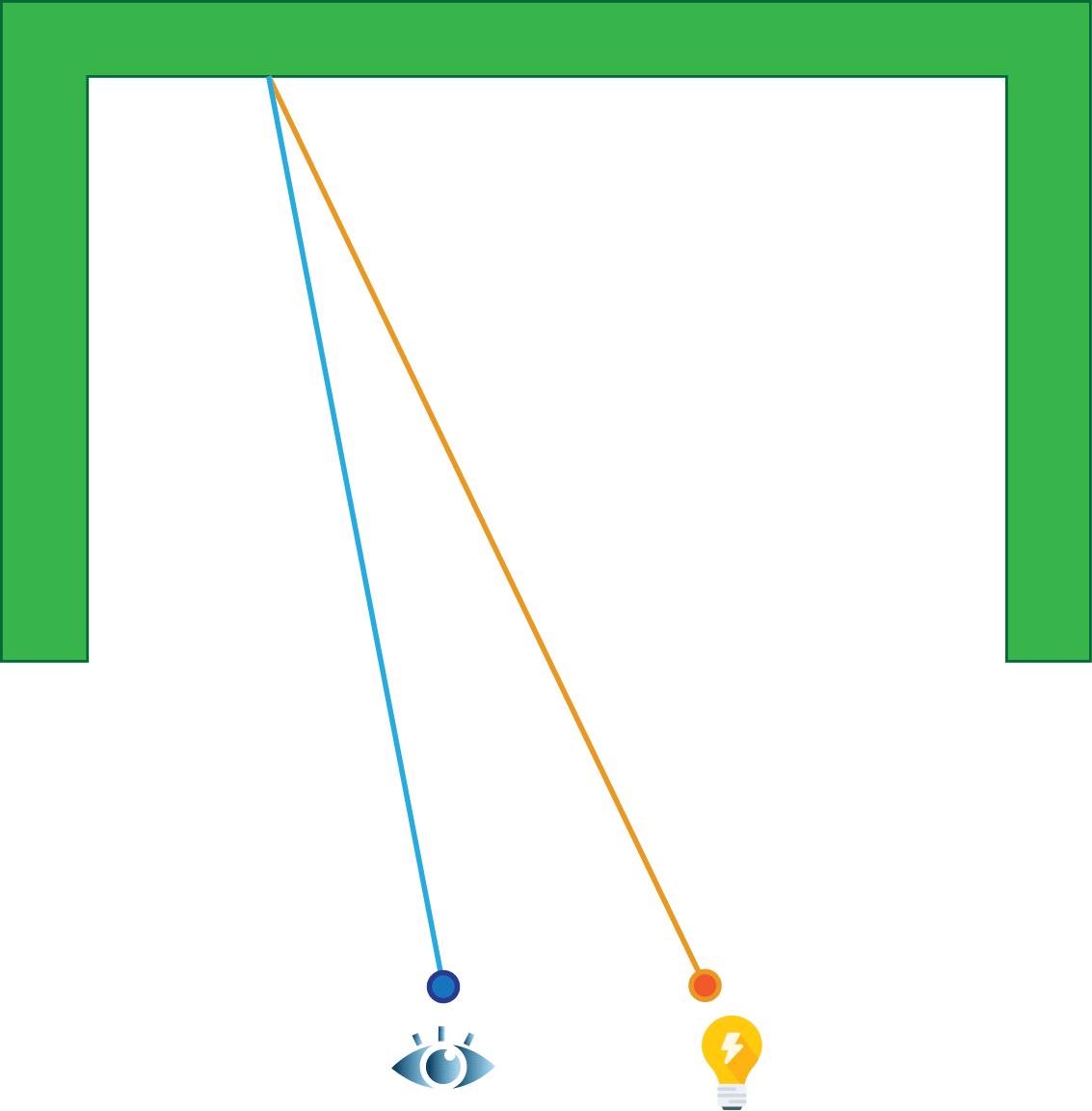
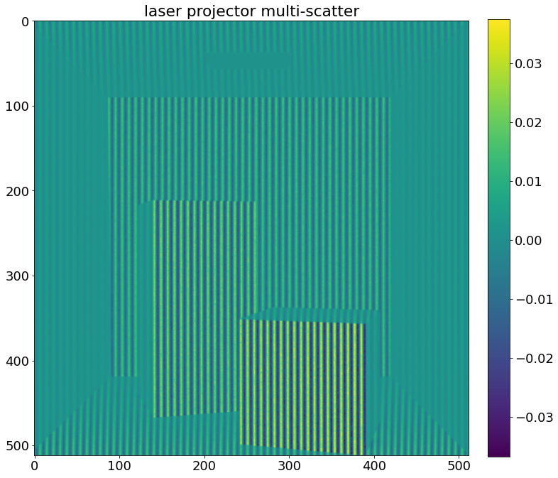
If we use the line-source-sweeping setup, one possible way to achieve this is by synchronizing the sensor with the sweeping of the light source: at each specific point of time, as the light source sweeps over the scene, only one column of pixels is activated. This will exclude the vast majority of multi-scatter light transport.

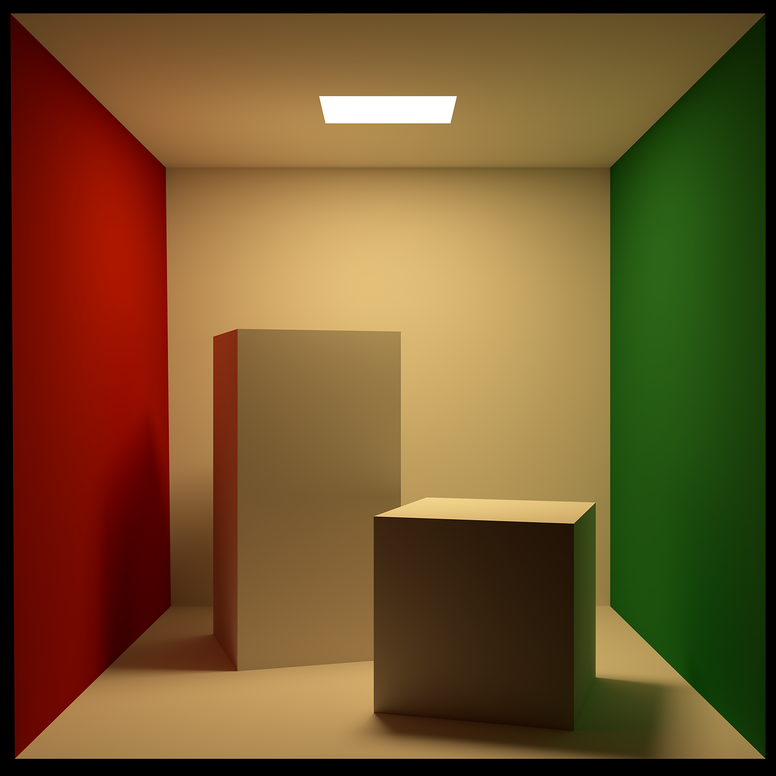
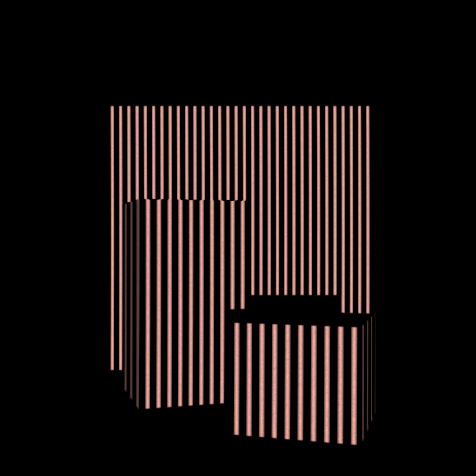
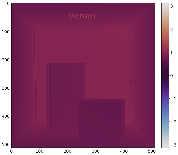
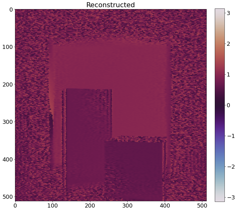
If we can synchronize the sensor with the light source, making only the corresponding line of pixels to be activated at any time, most multi-scatter light transport can be excluded.

At any instant, a single scanline of the sensor is active, and the illumination is confined to the corresponding region of the scene. The light source is temporally synchronized with the sensor’s rolling-shutter exposure so that the active illumination band and the sensing band coincide. In this way, we filtered out the unwanted multiple-scattering contribution (the width is exaggerated here for demonstration purpose).

Open lambertian scene

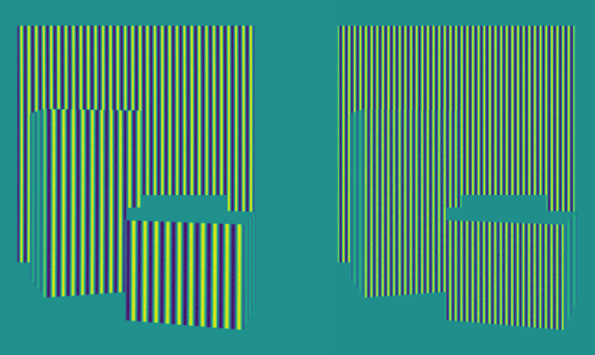
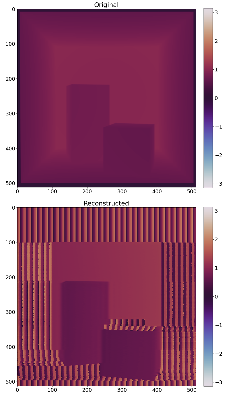
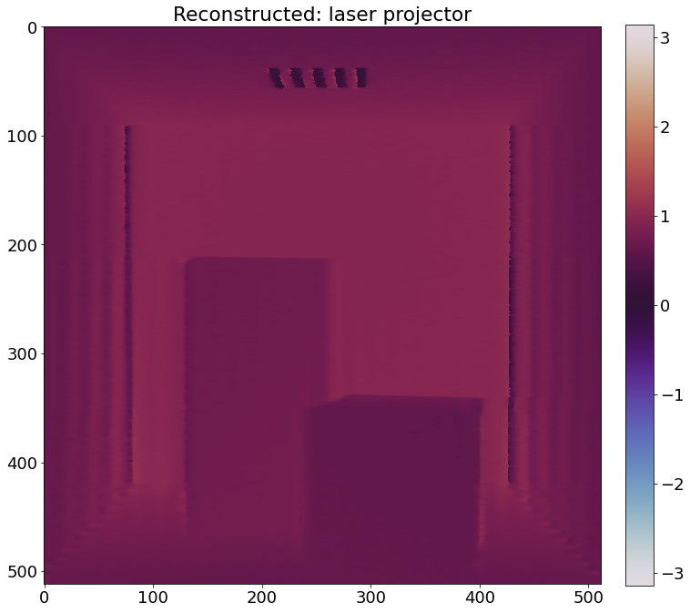
In the scene, every material is Lambertian and the scene is not closed (the whole wall on the side of the camera is removed). As a result, multi-scatter contribution is not so strong. In this case, although we can see some noticeable random noise, even without doing anything extra, we can reconstruct the depth without much trouble.

We can see the noise in this setup, though it's not too pronounced.

If we only visualize double-scattering, we can see the noise as expected (the original output was dark, the exposure was raised high for demonstration purpose).

The reconstructed result also looks noisy.

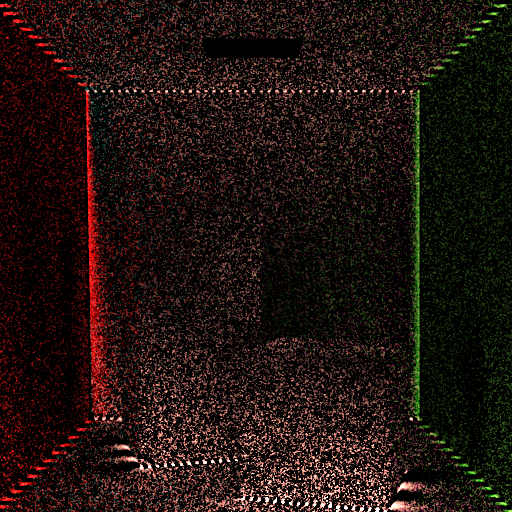
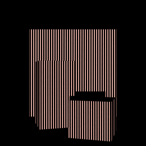
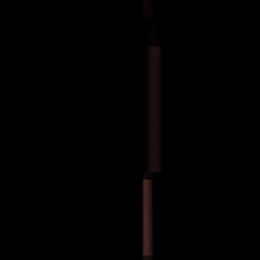
If we visualize only double-scatter, we can see the noise as expected, although it's really dark.

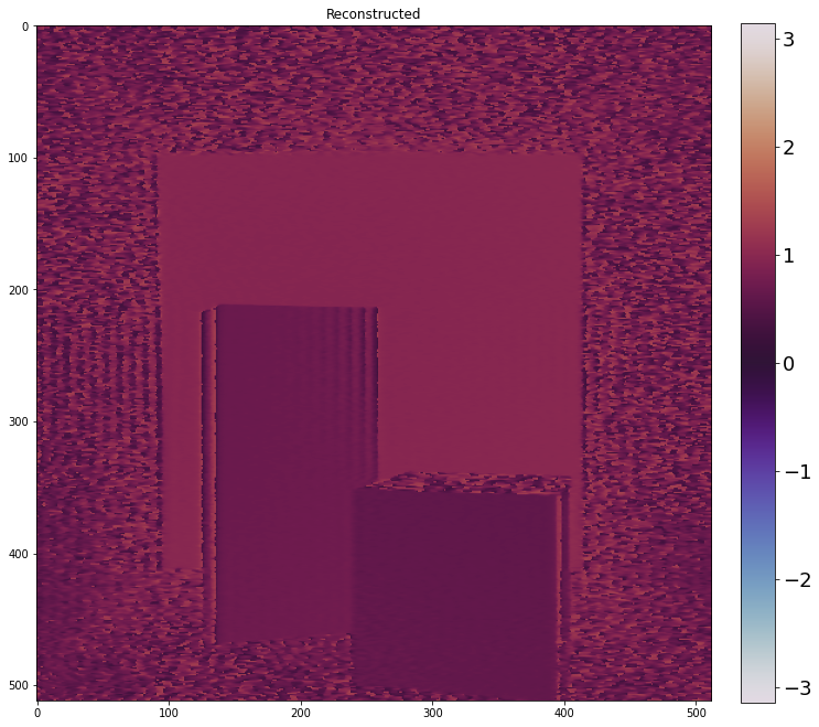
Closed, semi-specular, high-albedo scene

To make the multi-scatter contribution more pronounced, I added a different scene: the shape of the box is similar but the camera and light source are now inside. The material is a rough metal with really high albedo.

Left: single-scatter only; Right: multi-scatter enabled. With this setup, we see much more pronounced noise created by multi-scatter.

If only single-scatter is enabled, it works normally.

If we also enable multi-scatter, now large regions are covered by noise.

After synchronizing the shutter and the light source, most noise is removed.

If you synchronize the shutter with the sweeping line light projector, we get a lot of noise removed and the boundaries also become much clearer.

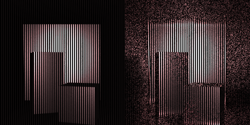
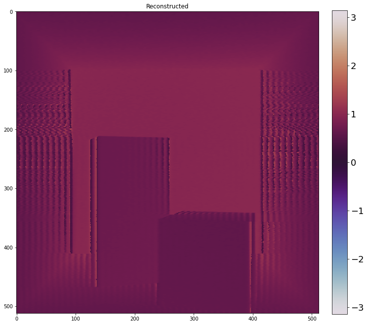
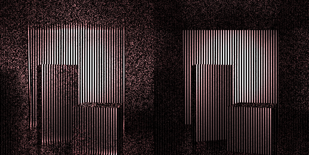
If we only look at double-scatter, we can see that after taking the correlation, instead of forming patterns, large regions will be covered with random noise, as expected.

Conclusions

This project shows that a CW time-of-flight (TOF) imaging system—normally requiring multiple phase-shifted exposures—can be reconfigured to recover depth and complex phase information from a single shot by leveraging principles from off-axis holography. Achieving this is far from straightforward: only a narrow class of spatiotemporal modulation patterns produces an isolatable heterodyne term, and many seemingly valid configurations fail due to subtle geometric and sampling constraints.

A key contribution of this work is identifying exactly which configurations work and why. We demonstrate that only setups imposing a spatially linear phase directly in image coordinates generate a clean, shiftable spectral component. Configurations that impose phase through illumination geometry (e.g., swept or offset laser patterns) break this alignment and cannot be salvaged by parameter tuning alone. These failure modes are rarely discussed but critically important for anyone attempting mixed spatiotemporal demodulation.

On the engineering side, the project introduces a general-purpose, time-resolved simulation framework capable of evaluating a wide family of modulation schemes. This required extending a path tracer with modulated emitters and sensors, rolling/global-shutter behavior, waveform-controlled demodulation, and per-pixel synchronization—tools that do not exist in standard rendering systems. The simulator makes it possible to probe subtle interactions between optical coding and light transport that would be extremely difficult to isolate on hardware.

Finally, we analyze and address a major practical obstacle: multi-scatter contamination. Through controlled experiments, we show how higher-order transport destroys the sinusoidal structure needed for holographic recovery, and we demonstrate that synchronizing illumination and sensor activation can suppress most of these contributions even in high-albedo scenes.