Laplace Transform Visualizer - Building Geometric Intuition

The Laplace transform is fundamental to control systems, signal processing, and differential equations—building geometric intuition makes these applications more accessible.

The Challenge

The Fourier transform has excellent visual intuitions: rotating vectors, periodic decomposition, frequency spectra (see the Fourier Art Generator). The Laplace transform is harder—it introduces growth, decay, and complex scaling that don't map as naturally to physical intuition.

This project experiments with interactive visual mappings to reveal how structure in the time domain is reflected in the s-domain. The visualizations work, but honestly still don't feel as intuitive as Fourier—this remains an open problem.

F(s) = ∫₀^∞ f(t)·e^(-st) dt    where s = σ + iω

Interactive Visualization

Note: This is a pre-rendered video from the original native implementation. The full interactive visualizer has not yet been ported to the web.

The Six-Panel Layout

This layout presents the Laplace transform through coordinated views, each revealing a different aspect of the computation:

Panel 1a (s-plane): Click and drag to adjust σ + iω—this is your "control surface" for exploring the transform
Panel 1b (f(t)): The original time-domain function before transformation
Panel 2a (Re/Im components): Real and imaginary parts of the integrand f(t)·e^(-st)—watch how changing s affects oscillation and decay
Panel 2b (Complex path): The trajectory traced by the integrand in the complex plane as t increases
Panel 3 (Riemann sum): The accumulating integral F(s)—rectangles sum to give the final transform value

The power is in the coordination: adjusting s in one panel immediately updates all others, revealing how the abstract integral formula manifests geometrically.

Global Operator View

Single s-value: detailed integrand view

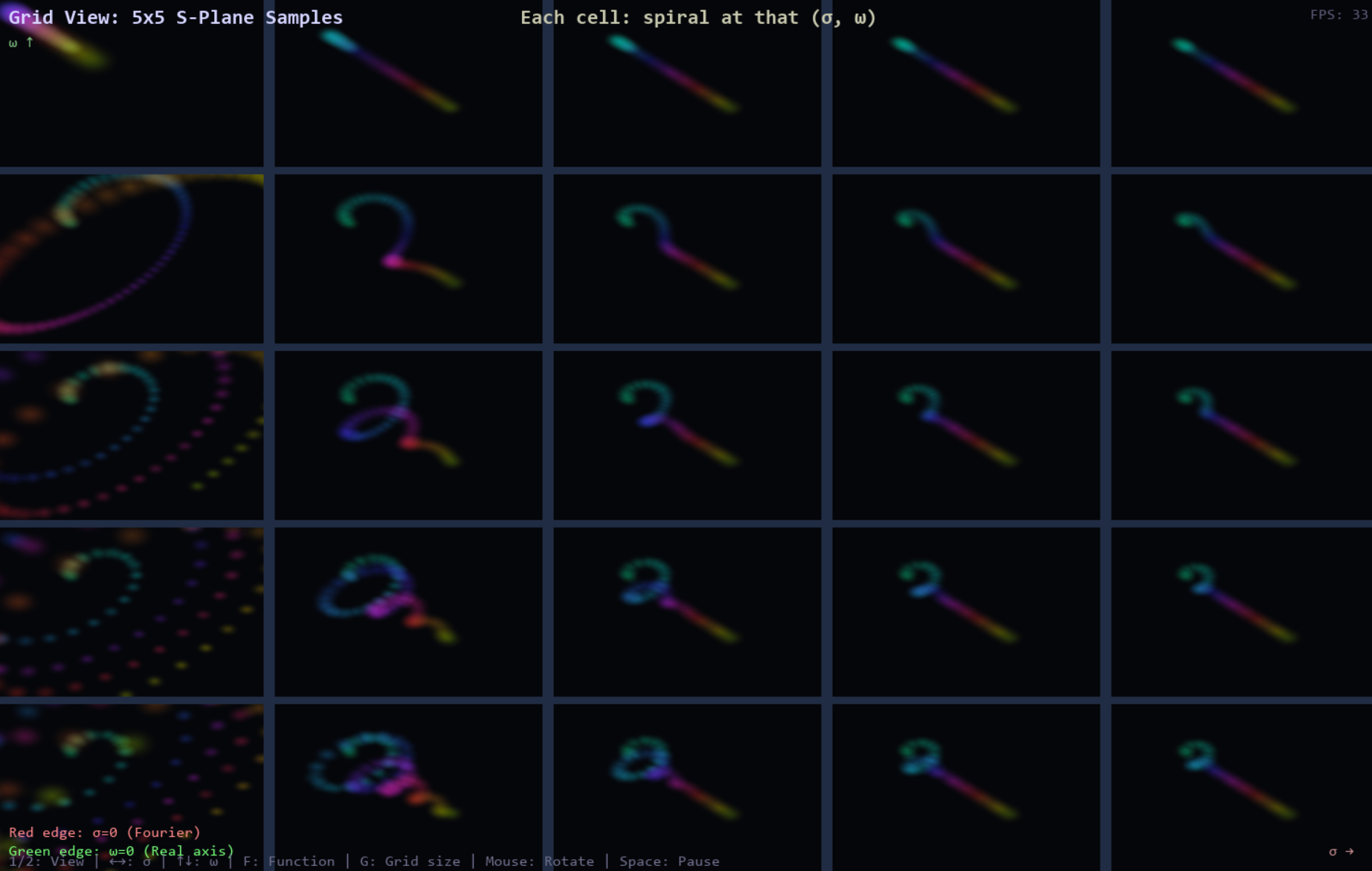
Grid view: transform evaluated across s-plane

The visualizer supports both detailed single-point analysis and a global view that evaluates the transform across a grid of s-values, revealing how oscillation, decay, and amplification interact across the complex plane.

Polarization Interpretation

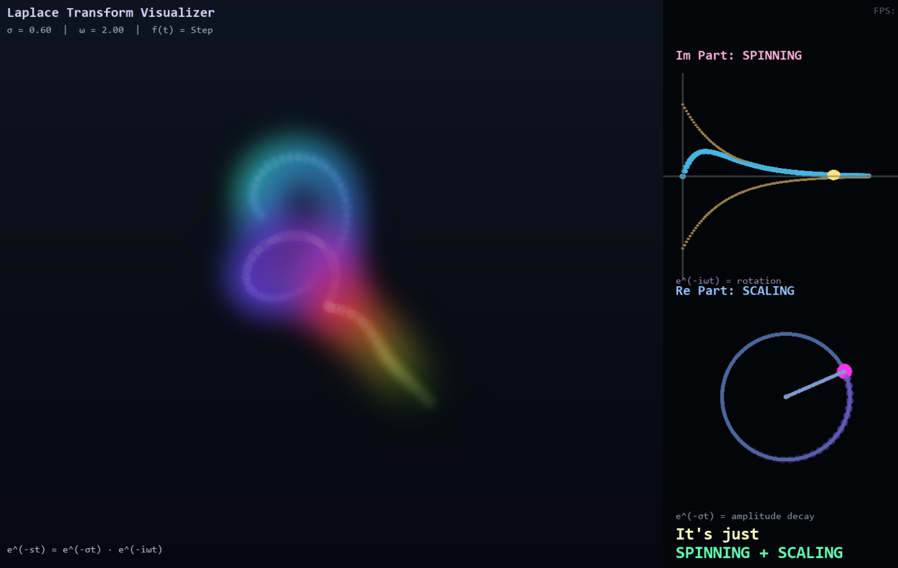
The Laplace Integrand as Polarized Motion

The Laplace integrand f(t)·e^−st, with s = σ + iω, can be interpreted geometrically as a trajectory in the complex plane.

The complex exponential decomposes as e^−st = e^−σt · e^−iωt, combining two distinct motions:

Rotation (e^−iωt): uniform phase rotation in the complex plane at angular frequency ω
Decay (e^−σt): a radially shrinking amplitude envelope with decay rate σ

Together, these generate a contracting spiral. When modulated by f(t), the resulting motion is analogous to elliptically polarized light with decaying intensity — a geometric, optics - inspired view.

Polarization visualization of Laplace integrand

The Laplace integrand visualized as polarized wave motion: rotation + decay creates spiraling trajectories in the complex plane.

How the Polarization Mode Works

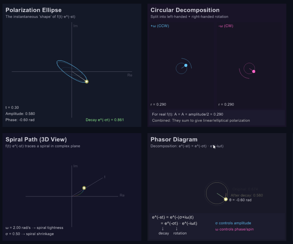
The visualizer displays four simultaneous views of the same integrand f(t)·e^(-st):

Polarization Ellipse: The instantaneous "shape" of the integrand. Size = |f(t)|·e^(-σt) (decaying amplitude), rotation = -ωt (phase). Shows a rotating, shrinking ellipse with fading history.
Circular Decomposition: Splits the motion into two counter-rotating circles—left-handed (+ω, counterclockwise) and right-handed (-ω, clockwise). For real f(t): both components have equal magnitude A₊ = A₋ = amplitude/2.
Spiral Path: The full 3D trajectory with time as depth. The spiral tightness is controlled by ω, shrinkage by σ.
Phasor Diagram: Shows the decomposition e^(-st) = e^(-σt) · e^(-iωt) with reference and decayed circles, plus the rotating phasor vector.

The Light Analogy

This connects directly to polarized light:

# Polarization decomposition (like optics)
Linear polarization  ↕  =  ↻ + ↺    (equal left + right circular)
Elliptical          ⬮  =  a·↻ + b·↺  (unequal components)
Circular            ↻  or  ↺        (pure single-handed rotation)

# For real f(t), the Laplace integrand is "linearly polarized":
f(t)·e^(-st) = A₊(t)·e^(-iωt) + A₋(t)·e^(+iωt)
               ↓                ↓
           Left-handed      Right-handed
           (positive ω)     (negative ω)

The two counter-rotating components sum to produce the observed linear/elliptical motion, just as left and right circularly polarized light combine to form other polarization states.

Generalizing the Spinner Model

Fourier's "rotating vector" intuition (the spinner) works because e^(-iωt) stays on the unit circle. The Laplace generalization allows the spinner to:

Shrink (σ > 0): spiral inward, converging to origin
Grow (σ < 0): spiral outward, diverging
Stay constant (σ = 0): pure rotation (Fourier case)

The Region of Convergence becomes visually intuitive: it's the set of σ values where the polarization ellipse shrinks to a point as t → ∞. The ellipse must decay—σ must be large enough to overcome any growth in f(t).

Fourier Scanline Interpretation

Status: This interpretation is less developed than the others—included here as a direction for future exploration.

One way to build intuition: the Fourier transform evaluates F(iω) = ∫f(t)e^(-iωt)dt—it samples along the imaginary axis of the s-plane.

The Laplace transform generalizes this to the entire complex plane. Each horizontal line s = σ + iω (fixed σ, varying ω) is like a "Fourier scanline" with an exponential envelope e^(-σt) applied first.

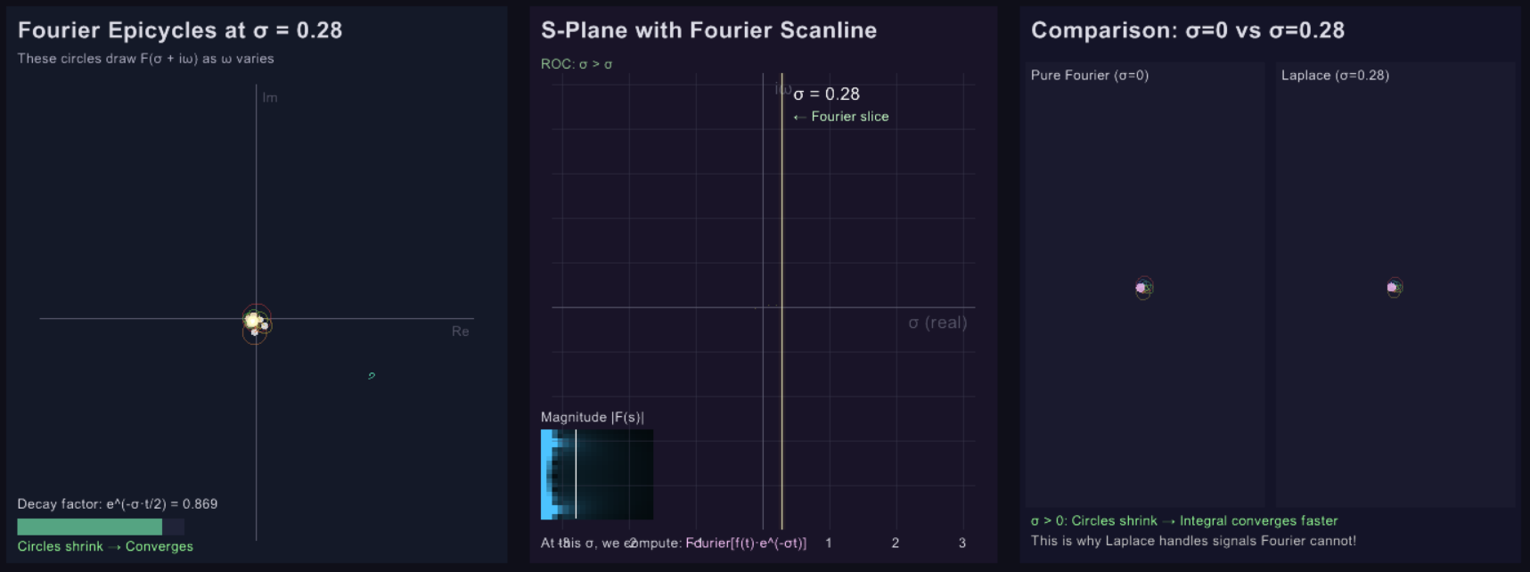
Visualizing the Laplace transform as Fourier analysis performed after exponential windowing. Different σ values reveal different aspects of the signal's structure.

The Idea

This perspective clarifies why the region of convergence matters: the integral only converges for σ values where e^(-σt) decays faster than f(t) grows. The Fourier transform (σ = 0) only works for bounded signals; Laplace extends to exponentially growing signals by "damping" them first.

# Fourier: only works if f(t) is bounded
F(iω) = ∫ f(t) · e^(-iωt) dt

# Laplace: works for exponentially growing f(t) if σ > growth rate  
F(σ + iω) = ∫ f(t) · e^(-σt) · e^(-iωt) dt
          = ∫ [f(t)·e^(-σt)] · e^(-iωt) dt   ← Fourier of damped signal

Future Directions

Planned Extensions

Inverse transform visualization: Contour integration in the s-plane
Pole-zero dynamics: Interactive exploration of system behavior
Transfer function view: Input → system → output with Laplace
Z-transform bridge: Connecting continuous and discrete domains

Project Status: This is an experimental/exploratory visualization project. The native Ruby implementation provides real-time interaction; web port is planned for future development. The goal is building intuition, not replacing formal analysis tools.