Symbolic Math Engine - Ruby Implementation

See It In Action

Watch a quick demonstration of the symbolic math engine handling a complex derivative (more demos: integral and simplification below):

How to Use the Interface

The web interface provides an intuitive workflow for symbolic computation:

1. Input Bar

Type a mathematical formula using standard notation and press Enter to parse it into the expression tree.

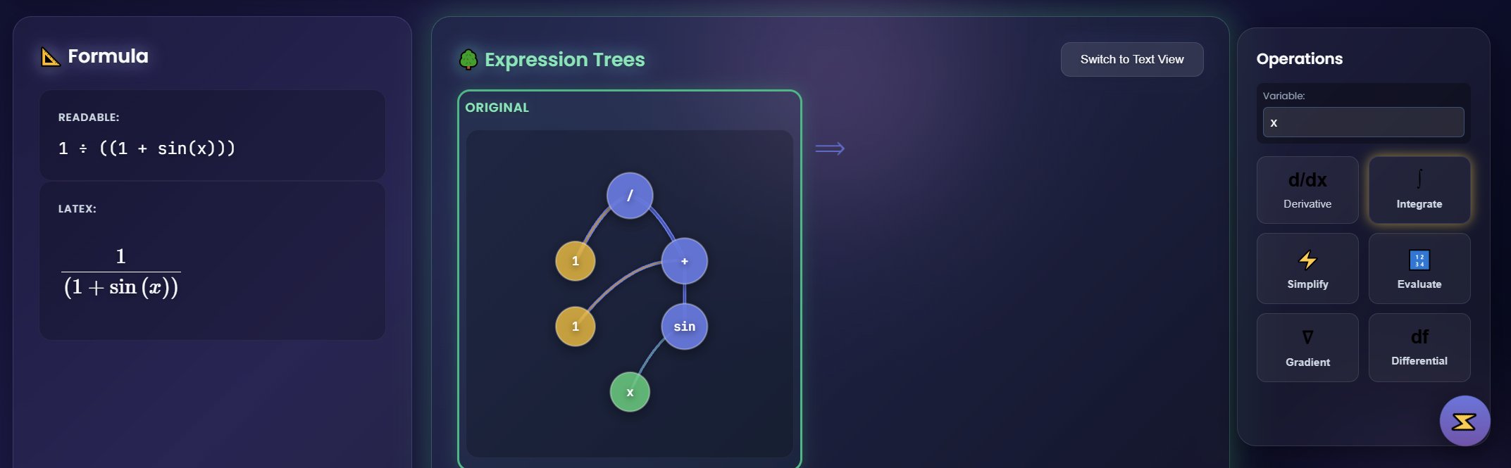
2. Tree View & Operations

Once entered, the original formula appears on the left as a tree structure. Choose operations from the right sidebar to proceed: differentiate, integrate, simplify, or evaluate.

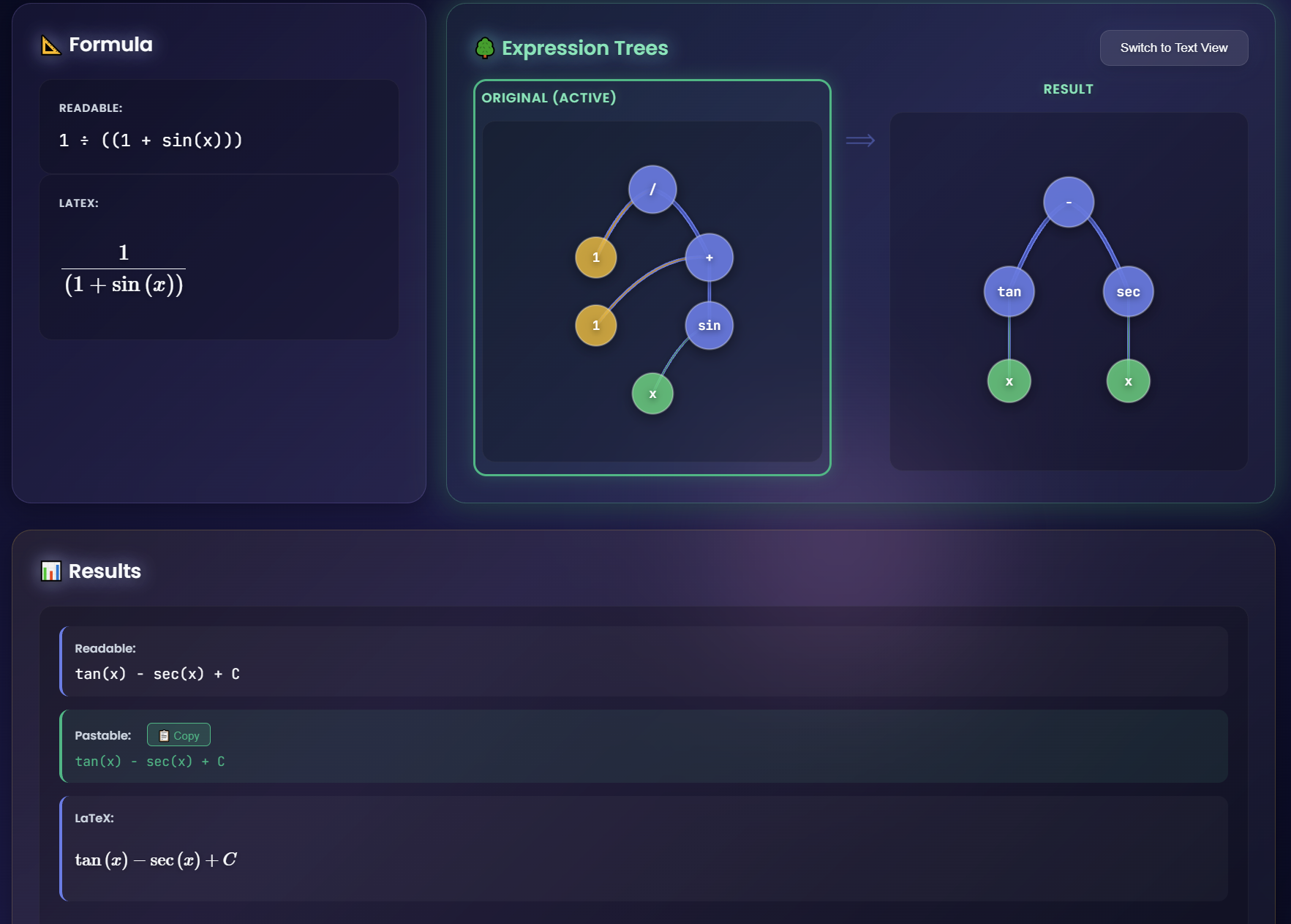
3. Result Display

The result is shown as a tree structure, written out in raw infix form, and beautifully rendered in LaTeX notation.

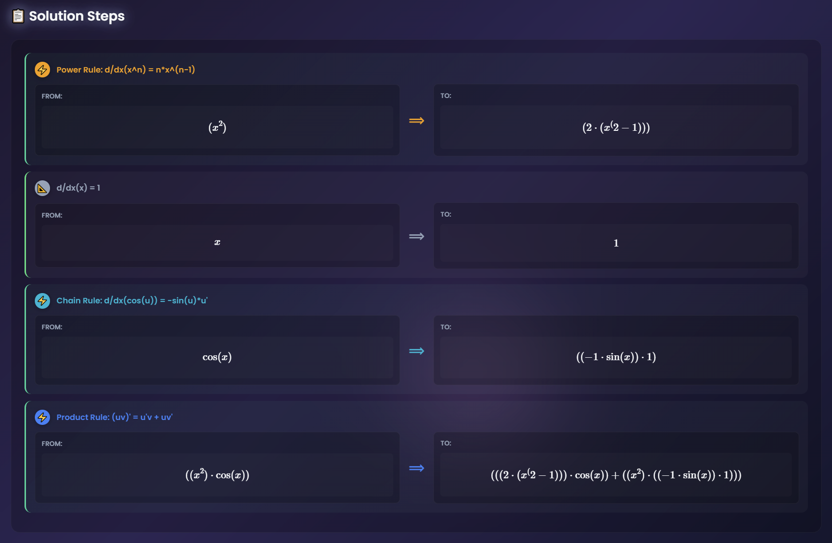
4. Step-by-Step View

Expand the steps section below to see every transformation applied during the computation, perfect for learning and debugging.

What It Can Do

🌲

Tree-Based Architecture

Expressions are represented as binary trees, where operators form internal nodes and operands form leaves. This elegant structure enables recursive algorithms for all operations.

∂

Symbolic Differentiation

Complete implementation of calculus rules: product rule, quotient rule, chain rule, and derivatives of all elementary functions. Handles arbitrary compositions.

∫

Heuristic Integration

Pattern-matching integration with algebraic simplification, by-parts detection, substitution, and partial fractions—covering common integral forms without a full decision procedure.

⚡

Smart Simplification

Iterative simplification engine with algebraic rules, constant folding, identity elimination, and experimental expansion strategies.

📐

Why Symbolic/Analytical? Numerical methods dominate practical computation, but analytical approaches unlock capabilities that numerical methods cannot provide: exact derivatives enable gradient-based optimization without discretization error; closed-form solutions reveal structural properties invisible to sampling; symbolic manipulation enables algebraic simplification before expensive evaluation. Even when fully analytical solutions are intractable, partially analytical pipelines—symbolic where possible, numerical where necessary—often outperform purely numerical approaches. Research on analytical solutions to rendering equations (achievable only in simplified setups) and automatic differentiation frameworks both demonstrate this principle: analytical treatment, even partial, provides leverage.

🔧

Why From the Ground Up? Existing CAS libraries (SymPy, Mathematica, Maple) are powerful but opaque. Building a symbolic engine from scratch provides direct insight into the comparative difficulty of each component: parsing is straightforward, differentiation follows mechanical rules, but integration requires sophisticated decision procedures (the Risch algorithm) that reveal deep connections between algebra and analysis. Understanding these internals—where the hard problems actually lie—informs how to design systems that combine symbolic and numerical computation effectively.

💎

Why Ruby? Ruby's elegant syntax and powerful metaprogramming capabilities make it ideal for implementing mathematical abstractions. The language's expressiveness allows the code to closely mirror mathematical notation.

⚠️

GitHub Pages Limitation: This project cannot be hosted live on GitHub Pages because the backend mathematical engine is written in Ruby (using Sinatra). GitHub Pages only supports static HTML/CSS/JavaScript. The original live demo required a Ruby server to handle symbolic computation requests.

System Architecture

Expression Tree Data Structure

At the core of the system is the ExpressionNode class, implementing a binary tree where:

Leaf nodes contain constants or variables
Internal nodes contain operators (+, -, ×, ÷, ^, sin, cos, ln, etc.)
Each node maintains pointers to left child, right child, and parent
Unary operators (sin, cos, ln) use only the right child

Ruby expression_node.rb

class ExpressionNode
  attr_accessor :isleaf, :data, :left, :right, :parent, :type
  
  def initialize(is_leaf, value)
    @isleaf = is_leaf
    @data = value.is_a?(Numeric) ? value : value.clone
    @left = nil
    @right = nil
    @parent = nil
    @type = nil
  end
  
  # Deep clone of node and its subtree
  def deep_clone
    new_node = ExpressionNode.new(@isleaf, @data)
    new_node.type = @type
    
    if @left
      new_node.left = @left.deep_clone
      new_node.left.parent = new_node
    end
    
    if @right
      new_node.right = @right.deep_clone
      new_node.right.parent = new_node
    end
    
    new_node
  end
  
  # Check if subtree is constant with respect to a variable
  def constant_wrt?(variable)
    return false unless self
    
    if @isleaf
      return @data != variable
    end
    
    left_const = @left ? @left.constant_wrt?(variable) : true
    right_const = @right ? @right.constant_wrt?(variable) : true
    
    return left_const && right_const
  end
end

The deep_clone method is crucial for derivative and integration operations, as it allows us to create independent copies of subtrees without modifying the original expression. The constant_wrt? method recursively checks if a subtree depends on a given variable, enabling optimization of integration and simplification routines.

Tree Visualization System

One of the most elegant parts of the codebase is the tree visualizer, which renders expression trees with beautiful Unicode formatting:

Ruby tree_visualizer.rb

def visualize_node(node, prefix, output, show_values, branch_type = "ROOT")
  return unless node
  
  # Node visualization with clear branch indicators
  if branch_type == "ROOT"
    output.print "  🌲 ROOT: "
  else
    output.print prefix
    if branch_type == "LEFT"
      output.print "├─[L]─ "
    else
      output.print "└─[R]─ "
    end
  end
  
  # Node content with styling
  if node.isleaf
    case node.data
    when Numeric
      output.print "【#{format_number(node.data)}】"
    when String
      if @variables.key?(node.data)
        value_str = show_values && @variables[node.data] ? "=#{@variables[node.data]}" : ""
        output.print "<#{node.data}#{value_str}>"
      else
        output.print "【#{node.data}】"
      end
    end
  else
    output.print "⟨#{node.data}⟩"
  end
  output.puts
  
  # Recursively display children with proper indentation
  if node.left || node.right
    new_prefix = branch_type == "ROOT" ? "  " : 
                 branch_type == "LEFT" ? prefix + "│      " : 
                                        prefix + "       "
    
    visualize_node(node.left, new_prefix, output, show_values, "LEFT") if node.left
    visualize_node(node.right, new_prefix, output, show_values, "RIGHT") if node.right
  end
end

Example Tree Output

  🌲 ROOT: ⟨+⟩
  ├─[L]─ ⟨*⟩
  │      ├─[L]─ 【2】
  │      └─[R]─ ⟨^⟩
  │             ├─[L]─ 
  │             └─[R]─ 【2】
  └─[R]─ ⟨*⟩
         ├─[L]─ 【3】
         └─[R]─

Expression: 2x² + 3x

Symbolic Differentiation

The derivative engine implements all fundamental calculus rules through recursive tree manipulation. Each operation creates a new subtree representing the derivative, following exact mathematical rules.

Core Differentiation Rules

Power Rule

$$\frac{d}{dx}(x^n) = n \cdot x^{n-1}$$

Product Rule

$$\frac{d}{dx}(uv) = u'v + uv'$$

Quotient Rule

$$\frac{d}{dx}\left(\frac{u}{v}\right) = \frac{u'v - uv'}{v^2}$$

Chain Rule

$$\frac{d}{dx}f(g(x)) = f'(g(x)) \cdot g'(x)$$

Implementation: Product Rule

The product rule implementation showcases the elegance of tree-based symbolic computation:

Ruby derivative_operations.rb

when '*'
  # Product rule: (uv)' = u'v + uv'
  u = node.left
  v = node.right
  u_prime = compute_derivative(u, variable, steps, aggressive_simplify)
  v_prime = compute_derivative(v, variable, steps, aggressive_simplify)
  
  # u'v term
  term1 = ExpressionNode.new(false, "*")
  term1.connect(u_prime, "L")
  term1.connect(v.deep_clone, "R")
  
  # uv' term
  term2 = ExpressionNode.new(false, "*")
  term2.connect(u.deep_clone, "L")
  term2.connect(v_prime, "R")
  
  # u'v + uv'
  result = ExpressionNode.new(false, "+")
  result.connect(term1, "L")
  result.connect(term2, "R")
  
  steps << {
    operation: "derivative", 
    rule: "Product Rule: (uv)' = u'v + uv'", 
    from: node.to_infix, 
    to: result.to_infix
  } if steps
  
  result

Advanced: General Power Rule

For the general case $f(x)^{g(x)}$, we use logarithmic differentiation. This is one of the more complex implementations:

Ruby derivative_operations.rb

# General case: f(x)^g(x) using logarithmic differentiation
# d/dx(f^g) = f^g * d/dx(g*ln(f)) = f^g * (g'*ln(f) + g*f'/f)

result = ExpressionNode.new(false, "*")
result.connect(node.deep_clone, "L")

# (g'*ln(f) + g*f'/f)
inner = ExpressionNode.new(false, "+")

# g' * ln(f)
term1 = ExpressionNode.new(false, "*")
term1.connect(compute_derivative(node.right, variable, steps, aggressive_simplify), "L")
ln_f = ExpressionNode.new(false, "ln")
ln_f.connect(node.left.deep_clone, "R")
term1.connect(ln_f, "R")

# g * f' / f
term2 = ExpressionNode.new(false, "*")
term2.connect(node.right.deep_clone, "L")
div_part = ExpressionNode.new(false, "/")
div_part.connect(compute_derivative(node.left, variable, steps, aggressive_simplify), "L")
div_part.connect(node.left.deep_clone, "R")
term2.connect(div_part, "R")

inner.connect(term1, "L")
inner.connect(term2, "R")
result.connect(inner, "R")

Mathematical Insight: For $f(x)^{g(x)}$, we can't use the simple power rule or exponential rule. Instead, we take the logarithm: $\ln(y) = g(x)\ln(f(x))$, then differentiate implicitly: $\frac{1}{y}\frac{dy}{dx} = g'(x)\ln(f(x)) + g(x)\frac{f'(x)}{f(x)}$, giving us $\frac{dy}{dx} = f(x)^{g(x)}\left[g'(x)\ln(f(x)) + g(x)\frac{f'(x)}{f(x)}\right]$.

Derivative Demonstrations

Complex Hand-Typed Derivative

Watch the engine handle a complex derivative typed by hand:

An Even More Complex Derivative

The system handles arbitrarily nested compositions. Here's a significantly more complex example:

More Derivatives in Action

Here are additional examples showing consistent behavior across different function types:

✓

All derivatives can be solved regardless of complexity. The recursive tree-based algorithm handles arbitrary compositions of functions, applying the chain rule, product rule, and quotient rule as needed.

Symbolic Integration

Integration is significantly more complex than differentiation. The system uses a heuristic pattern-matching approach:

Core Rules

Direct Integration

Handles standard forms using known antiderivatives:

Power rule: $\int x^n dx = \frac{x^{n+1}}{n+1}$
Trigonometric and exponential forms
Sum/difference and constant multiple rules
Logarithmic patterns

Advanced

Transformation Techniques

Pattern detection and algebraic manipulation:

Integration by parts (LIATE heuristic)
Substitution detection
Partial fraction decomposition
Trigonometric power reduction

🔬

Why Not Full RISCH?

The Risch algorithm is completely deterministic and can even determine whether a function has an elementary antiderivative. However, implementing the full algorithm is extraordinarily complex—even Mathematica doesn't have a complete RISCH implementation. A theoretically perfect and complete Risch algorithm is considered practically impossible to implement in its full generality.

This project takes a pragmatic approach: using pattern matching and heuristic methods inspired by Risch's ideas, achieving good coverage of common integrals without the overwhelming complexity of the full algorithm.

Term Rewriting: A Practical Alternative

Instead of implementing the full Risch algorithm, this system uses a term rewriting approach—fundamentally the same technique used in chess engines and Monte Carlo ray tracing:

♟️

The Search Space Analogy

A chess engine explores possible moves; a ray tracer samples possible light paths; this integrator explores possible algebraic transformations. Each applies local rewrite rules (subtree substitutions) and evaluates whether the result is "better" by some heuristic.

🎲

Non-Deterministic Exploration

Unlike Risch's deterministic decision procedure, this stochastic approach explores multiple transformation paths. When one path fails, it backtracks and tries another—trading theoretical completeness for practical coverage of common cases.

Ruby simplification.rb (conceptual)

# Term rewriting = recursive subtree substitution
def apply_rewrite_rules(node, steps)
  changed = false
  
  # Each rule: pattern → replacement
  changed |= apply_rule(node, "x + x", "2*x")      # Combine like terms
  changed |= apply_rule(node, "x * x", "x^2")      # Power conversion
  changed |= apply_rule(node, "(x^a)^b", "x^(a*b)") # Power of power
  changed |= apply_rule(node, "x - x", "0")        # Cancellation
  
  # Recursively apply to children
  changed |= apply_rewrite_rules(node.left, steps) if node.left
  changed |= apply_rewrite_rules(node.right, steps) if node.right
  
  # Iterate until no more changes (fixed point)
  changed
end

✓

Practical Results: Despite being theoretically incomplete, this approach already handles many non-trivial integrals: products of exponentials and trigonometrics (e.g., ∫e^x·sin(x)dx), rational functions, inverse trig functions, and nested compositions. The heuristic-driven exploration succeeds where a naive algebraic approach would fail.

Pattern Detection System

The experimental integrator uses sophisticated pattern matching with colored terminal output for debugging:

Ruby experimental_risch.rb

module StepVisualizer
  def self.print_pattern(description, color = Colors::BRIGHT_BLUE)
    msg = "│ 🔍 Pattern: #{description}"
    ExperimentalRisch.log_debug("#{color}#{msg}#{Colors::RESET}", level: 0)
  end
  
  def self.print_method(method_name, color = Colors::BRIGHT_GREEN)
    msg = "│ ⚡ Method: #{method_name}"
    ExperimentalRisch.log_debug("#{color}#{msg}#{Colors::RESET}", level: 0)
  end
  
  def self.print_step(label, value, color = Colors::BRIGHT_YELLOW)
    msg = "│ ├─ #{label}: #{value}"
    ExperimentalRisch.log_debug("#{color}#{msg}#{Colors::RESET}", level: 0)
  end
  
  def self.print_result(result, color = Colors::BRIGHT_PURPLE)
    msg = "│ ✓ Result: #{result}"
    ExperimentalRisch.log_debug("#{color}#{msg}#{Colors::RESET}", level: 0)
  end
end

Integration Techniques by Test Case

Polynomial Integration Power Rule

$$\int (2x^2 + 3x + 1) \, dx = \frac{2x^3}{3} + \frac{3x^2}{2} + x + C$$

Handles arbitrary polynomial degrees by recursively applying the power rule to each term.

Trigonometric Integration Pattern Matching

$$\int \sin(x) \, dx = -\cos(x) + C$$ $$\int \cos(x) \, dx = \sin(x) + C$$ $$\int \sec^2(x) \, dx = \tan(x) + C$$

Recognizes standard trigonometric forms and applies known antiderivatives.

Rational Functions Algebraic Simplification

$$\int \frac{x}{x^2} \, dx = \int \frac{1}{x} \, dx = \ln|x| + C$$

Simplifies rational expressions before integration, canceling common factors.

Substitution Detection Experimental

$$\int 2x \cdot e^{x^2} \, dx \rightarrow u = x^2, du = 2x \, dx$$ $$= \int e^u \, du = e^{x^2} + C$$

Automatically detects when a composition suggests u-substitution.

Rational Fraction Handling

A subtle but important detail: the system preserves exact rational representations to avoid floating-point errors:

Ruby integration_operations.rb

def create_rational_fraction(numerator_val, denominator_val)
  # Check if division produces a clean decimal
  if denominator_val != 0 && is_clean_decimal?(numerator_val, denominator_val)
    # Create as evaluated number
    result = numerator_val.to_f / denominator_val.to_f
    return ExpressionNode.new(true, result)
  else
    # Keep as fraction
    fraction = ExpressionNode.new(false, "/")
    fraction.connect(ExpressionNode.new(true, numerator_val), "L")
    fraction.connect(ExpressionNode.new(true, denominator_val), "R")
    return fraction
  end
end

def is_clean_decimal?(num, den)
  return false if den == 0
  
  num_int = num.to_f == num.to_i.to_f ? num.to_i : num
  den_int = den.to_f == den.to_i.to_f ? den.to_i : den
  
  return true unless num_int.is_a?(Integer) && den_int.is_a?(Integer)
  
  # Check if denominator only has factors of 2 and 5 (terminating decimal)
  den_reduced = den_int.abs
  den_reduced /= 2 while den_reduced % 2 == 0
  den_reduced /= 5 while den_reduced % 5 == 0
  
  # If only 1 remains, it's a terminating decimal
  den_reduced == 1
end

Why This Matters: When integrating $\int x \, dx = \frac{x^2}{2}$, we want to keep it as $\frac{1}{2} \cdot x^2$ in symbolic form, not convert to $0.5 \cdot x^2$. This preserves exactness and produces cleaner LaTeX output. However, for $\frac{1}{4}$ (which equals 0.25), the system uses the decimal since it terminates cleanly.

Integration Demonstrations

Simple Integral Examples

Watch the system handle straightforward integration problems with algebraic and trigonometric functions:

Complex Integral with Pattern Detection

Here's a more challenging integral where the experimental Risch-like algorithm identifies patterns and applies substitution techniques:

Expression Simplification

Without simplification, symbolic operations quickly produce unwieldy expressions. Consider differentiating $x^3$ using the product rule three times—you'd get $x \cdot x \cdot 1 + x \cdot 1 \cdot x + 1 \cdot x \cdot x$ instead of $3x^2$. The simplification engine prevents this explosion.

Why Simplification is Critical

Without Simplification

$$\frac{d^2}{dx^2}(x^4) = ((4 \cdot x^{4-1}) \cdot 1) \cdot (4-1) \cdot x^{(4-1)-1}$$

→ Simplify →

With Simplification

$$\frac{d^2}{dx^2}(x^4) = 12x^2$$

Two-Tier Simplification System

Ruby simplification.rb

def simplify(track_steps: false, max_iterations: 30)
  puts "\n========================================="
  puts "STARTING SIMPLIFICATION"
  puts "Expression: #{@root.to_infix}"
  puts "Mode: #{@use_experimental_simplification ? 'Experimental' : 'Standard'}"
  puts "=========================================\n"
  
  steps = [] if track_steps
  iteration = 0
  changed = true
  last_expr = @root.to_infix
  
  while changed && iteration < max_iterations
    iteration += 1
    current_expr = @root.to_infix
    
    if @use_experimental_simplification
      changed = experimental_simplify_pass(@root, steps)
    else
      changed = standard_simplify_pass(@root, steps)
    end
    
    new_expr = @root.to_infix
    
    # Detect infinite loop
    if new_expr == last_expr && changed
      puts "  ⚠️  WARNING: Expression unchanged, stopping to prevent infinite loop"
      changed = false
    end
    
    last_expr = current_expr
  end
  
  puts "\nFINAL RESULT: #{@root.to_infix}"
  self
end

Standard Simplification Rules

Identity Elimination

$x + 0 = x$
$x \times 1 = x$
$x^1 = x$

Zero Absorption

$x \times 0 = 0$
$x^0 = 1$
$0 - x = -x$

Constant Folding

$2 + 3 = 5$
$4 \times 5 = 20$
$2^3 = 8$

Cancellation

$(a + c) - c = a$
$\frac{x^n}{x} = x^{n-1}$
$\frac{a \cdot x}{x} = a$

Experimental: Algebraic Expansion

The experimental mode includes expansion rules for common algebraic identities:

Ruby simplification.rb - Binomial Expansion

# Expand (x+a)^2 → x^2 + 2*x*a + a^2
if node.data == '^' && node.right && node.right.isleaf && 
   node.right.data.is_a?(Numeric) && node.right.data == 2 &&
   node.left && node.left.data == '+'
  
  u = node.left.left
  v = node.left.right
  
  if u && v
    # Build u^2
    u_squared = ExpressionNode.new(false, "^")
    u_squared.connect(u.deep_clone, "L")
    u_squared.connect(ExpressionNode.new(true, 2), "R")
    
    # Build 2*u*v
    two_uv = ExpressionNode.new(false, "*")
    two_uv.connect(ExpressionNode.new(true, 2), "L")
    uv_node = ExpressionNode.new(false, "*")
    uv_node.connect(u.deep_clone, "L")
    uv_node.connect(v.deep_clone, "R")
    two_uv.connect(uv_node, "R")
    
    # Build v^2
    v_squared = ExpressionNode.new(false, "^")
    v_squared.connect(v.deep_clone, "L")
    v_squared.connect(ExpressionNode.new(true, 2), "R")
    
    # Build u^2 + 2*u*v
    sum1 = ExpressionNode.new(false, "+")
    sum1.connect(u_squared, "L")
    sum1.connect(two_uv, "R")
    
    # Build (u^2 + 2*u*v) + v^2
    result = ExpressionNode.new(false, "+")
    result.connect(sum1, "L")
    result.connect(v_squared, "R")
    
    replace_node_with(node, result)
    steps << {
      operation: "simplification", 
      rule: "Expand: (u+v)^2 = u^2 + 2*u*v + v^2"
    } if steps
    changed = true
  end
end

Supported Expansions

$$(u + v)^2 = u^2 + 2uv + v^2$$

$$(u - v)^2 = u^2 - 2uv + v^2$$

$$(u + v)^3 = u^3 + 3u^2v + 3uv^2 + v^3$$

$$(u - v)^3 = u^3 - 3u^2v + 3uv^2 - v^3$$

$$a(b + c) = ab + ac$$

The Simplification Dilemma

Interestingly, "simplified" is context-dependent. Is $(x+1)^2$ simpler than $x^2 + 2x + 1$? The factored form is more compact, but the expanded form is easier for polynomial operations. The system makes trade-offs based on tree depth and operation counts.

Simplification in Action

Watch how the iterative simplification engine reduces complex expressions step by step, applying multiple rules in sequence:

Additional Features

Expression Evaluation

With the tree structure, evaluation is trivial—a simple post-order traversal:

Ruby expression_node.rb

def evaluate(var_values)
  return 0 unless self
  
  if @isleaf
    case @data
    when Numeric
      return @data.to_f
    when String
      return var_values[@data].to_f if var_values[@data]
      return 0.0
    end
  end
  
  # Operator evaluation
  case @data
  when '+'
    return @left.evaluate(var_values) + @right.evaluate(var_values)
  when '-'
    return @left.evaluate(var_values) - @right.evaluate(var_values)
  when '*'
    return @left.evaluate(var_values) * @right.evaluate(var_values)
  when '/'
    right_val = @right.evaluate(var_values)
    return right_val != 0 ? @left.evaluate(var_values) / right_val : Float::INFINITY
  when '^'
    return @left.evaluate(var_values) ** @right.evaluate(var_values)
  when 'sin'
    return Math.sin(@right.evaluate(var_values))
  when 'cos'
    return Math.cos(@right.evaluate(var_values))
  # ... more functions
  end
end

Vector Calculus Operations

The system extends to multivariable calculus with gradient, Laplacian, and differential form computations:

Gradient

$$\nabla f = \left(\frac{\partial f}{\partial x}, \frac{\partial f}{\partial y}, \frac{\partial f}{\partial z}\right)$$

Laplacian

$$\nabla^2 f = \frac{\partial^2 f}{\partial x^2} + \frac{\partial^2 f}{\partial y^2} + \frac{\partial^2 f}{\partial z^2}$$

Differential Form

$$df = \frac{\partial f}{\partial x}dx + \frac{\partial f}{\partial y}dy + \frac{\partial f}{\partial z}dz$$

Gradient Computation

The gradient operation computes partial derivatives with respect to multiple variables simultaneously:

Expression Evaluation

Evaluate expressions with specific variable values, perfect for numerical analysis and verification:

Tree View Modes: Graphical vs. Text

The interface supports two tree visualization modes: a graphical node-based view and a text-based hierarchical view. Each has distinct advantages:

Switching Between Views

When Text View is Handy

Machine Processing: Text tree format is easily parseable by other programs or scripts for automated analysis
Debugging: Quickly spot structural issues by reading the tree hierarchy without visual clutter
Copy-Paste: Export tree structure to documentation, reports, or code comments
Compact Representation: View deeply nested expressions without requiring large screen space
Version Control: Track changes to expression structure in text-based diff tools
API Integration: Feed tree representation directly into other symbolic computation tools

LaTeX Output Generation

For presentation, the system converts expression trees to beautiful LaTeX notation:

Ruby tree_visualizer.rb

def to_latex(node = nil, parent_op = nil)
  node = @root if node.nil?
  return "" unless node
  
  if node.isleaf
    if node.data.is_a?(Numeric)
      if node.data.to_f == node.data.to_i.to_f
        return node.data.to_i.to_s
      else
        # Convert to fraction for LaTeX
        rational = node.data.rationalize(1e-10)
        numerator = rational.numerator
        denominator = rational.denominator
        
        if denominator != 1 && denominator <= 1000
          return "\\frac{#{numerator}}{#{denominator}}"
        else
          return node.data.to_s
        end
      end
    else
      return node.data.to_s
    end
  end
  
  result = case node.data
  when '+'
    "#{to_latex(node.left, '+')} + #{to_latex(node.right, '+')}"
  when '/'
    "\\frac{#{to_latex(node.left, '/')}}{#{to_latex(node.right, '/')}}"
  when '^'
    base = to_latex(node.left, '^')
    "{#{base}}^{#{to_latex(node.right, '^')}}"
  when 'sin'
    "\\sin\\left(#{to_latex(node.right)}\\right)"
  when 'sqrt'
    "\\sqrt{#{to_latex(node.right)}}"
  # ... more cases
  end
  
  result
end

Example Outputs

Input: "x^2 + 2*x + 1"

$$x^2 + 2x + 1$$

Input: "sin(x)^2 + cos(x)^2"

$$\sin^2(x) + \cos^2(x)$$

Input: "(x^3)/3"

$$\frac{x^3}{3}$$

Input: "sqrt(x^2 + y^2)"

$$\sqrt{x^2 + y^2}$$

Comprehensive Test Suite

The project includes extensive testing across all features:

∂

Derivatives

Compositions, products, chains

∫

Basic Integrals

8 cases

∫

By Parts

4 cases

∫

Trig Powers

9 cases

∫

Partial Fractions

4 cases

∫

Trig Substitution

3 cases

∫

Advanced

10+ cases

⚡

Simplification

Algebraic, trig identities

Technical Notes

🏗️

Built from Scratch

No external CAS libraries—every algorithm implemented from first principles, following classical symbolic computation literature.

🌳

Uniform Tree Operations

Differentiation, integration, and simplification share the same recursive pattern: inspect node type, transform children, combine results. One traversal structure handles all symbolic operations.

🔬

Heuristic Integration

Pattern matching and term rewriting handle common integral forms—polynomials, trig powers, by-parts candidates, partial fractions—without requiring a full decision procedure.

🎨

Informative Visualization

Expression trees rendered as ASCII art or graphical output; derivation steps traced and exportable, making the engine's reasoning transparent and easy to communicate.

⚙️

Production-Ready API

Sinatra web server with RESTful endpoints, JSON responses, and interactive web interface.

🧪

Comprehensive Testing

30+ test cases covering edge cases, complex compositions, and multivariable calculus.

About This Showcase

This document presents a Ruby-based symbolic mathematics engine that implements core computer algebra system functionality. While the live demo cannot be hosted on GitHub Pages due to the Ruby backend requirement, the codebase demonstrates sophisticated algorithmic techniques and clean software architecture. The implementation serves as both a practical tool and an educational resource for understanding how symbolic computation works under the hood.

Project Highlights: Tree-based expression representation, recursive differentiation with all calculus rules, experimental Risch-like integration algorithm, iterative simplification with algebraic identities, LaTeX and Unicode output generation, and comprehensive vector calculus support.