Representation and Evolution in Five Dimensions
How high-dimensional data can evolve through changes in representation
Beyond Static Visualization
This project explores how high-dimensional data can evolve through changes in representation. It begins with a procedural five-dimensional field, where spatial, temporal, and latent axes are treated symmetrically and mapped to color. Distinct views are formed through slicing and projection, visualized via ray marching.
The key insight: fixing temporal and latent dimensions yields a concrete 3D field, but the act of viewing introduces new degrees of freedom. Representation shifts from (x,y,z,w,t) → RGBA to (x,y,z) + view direction → RGBA, effectively trading latent dimensions for angular ones.
This reframing opens two parallel paths for evolution: NeRF-style neural representations as a resampling mechanism, and Taichi-based diffusion dynamics operating on slices of the field.
5D Procedural Field Exploration
The base system generates structure in five dimensions via an iterated nonlinear mapping. By choosing which dimensions map to XYZ, which serves as time, and which as a navigable latent axis, the same underlying field produces radically different visual behavior.
Evolution via Taichi Diffusion
The Challenge: Evolving Procedural Data
A procedural field is defined by a function—it has no persistent state to modify. You can't "write" to a purely procedural volume. So how can we introduce evolution and feedback?
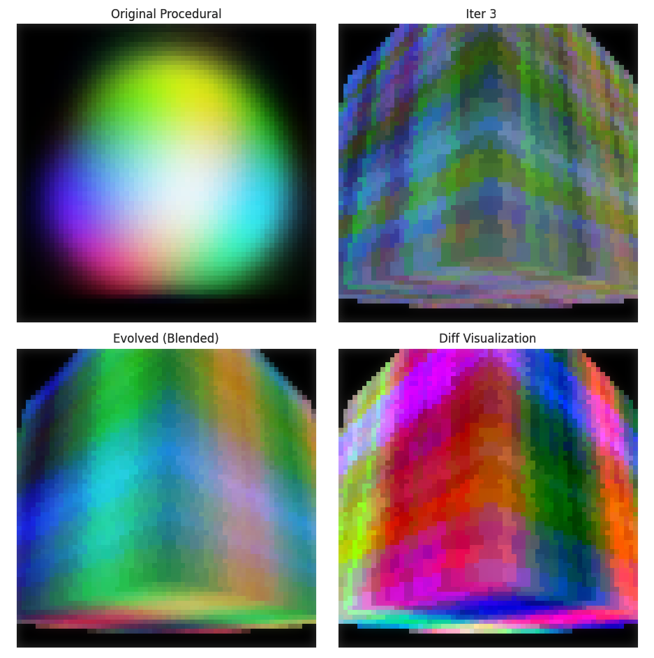
The solution: sample the procedural field into a discrete 3D tensor, run simulation dynamics on that slice, and track the difference between the evolved state and the original procedural values. This difference field becomes the medium for evolution.
Reaction-Diffusion on Sliced Data
Using Taichi for GPU-accelerated computation, the system samples a 3D slice from the 5D field at fixed (W, T) values, then applies reaction-diffusion dynamics:
# Sample 3D slice from 5D procedural field
slice = sample_5d_field(w=current_w, t=current_t)

# Initialize simulation state from procedural density
state = init_from_procedural(slice)

# Run Gray-Scott / SmoothLife dynamics
for step in range(n_steps):
    state = diffusion_step(state, slice)  # procedural modulates feed rate

# Track deviation from original
deviation = state - slice  # This is what "evolved"
The procedural field seeds and modulates the simulation, while the simulation's deviation from the original becomes a form of learned or evolved structure.
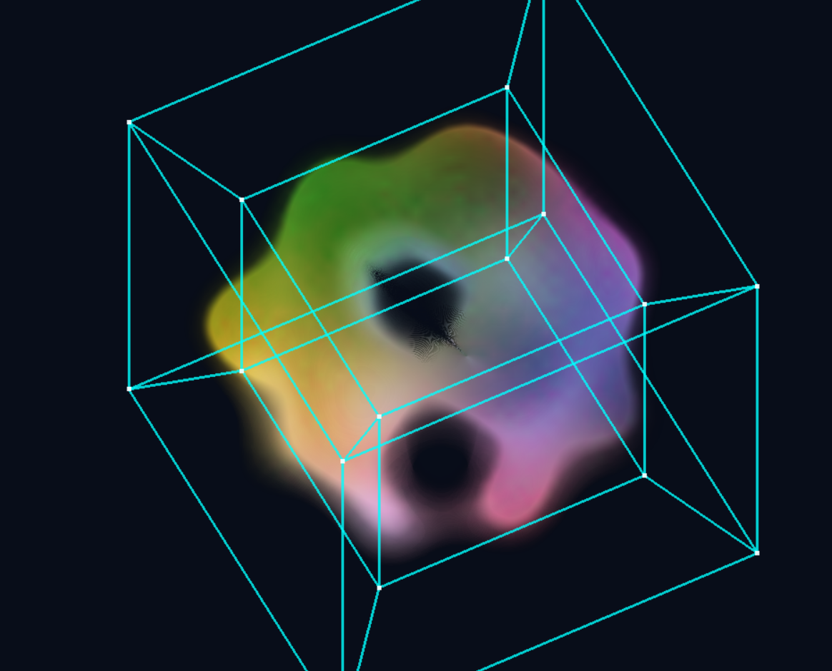
Gray-Scott reaction-diffusion running on a sampled slice, with the procedural field modulating local feed rates. Organic patterns emerge from the interplay.
Arbitrary Slicing: Beyond Canonical Axes
Rather than examining the 5D field through orthogonal slices—choosing three of the five canonical axes as XYZ—the implementation supports arbitrary slicing: cutting along any 3D hyperplane through the 5D space.
This transforms navigation from discrete axis-swapping into a continuous, geometry-driven process—smoothly rotating through higher-dimensional space rather than jumping between axis-aligned perspectives.
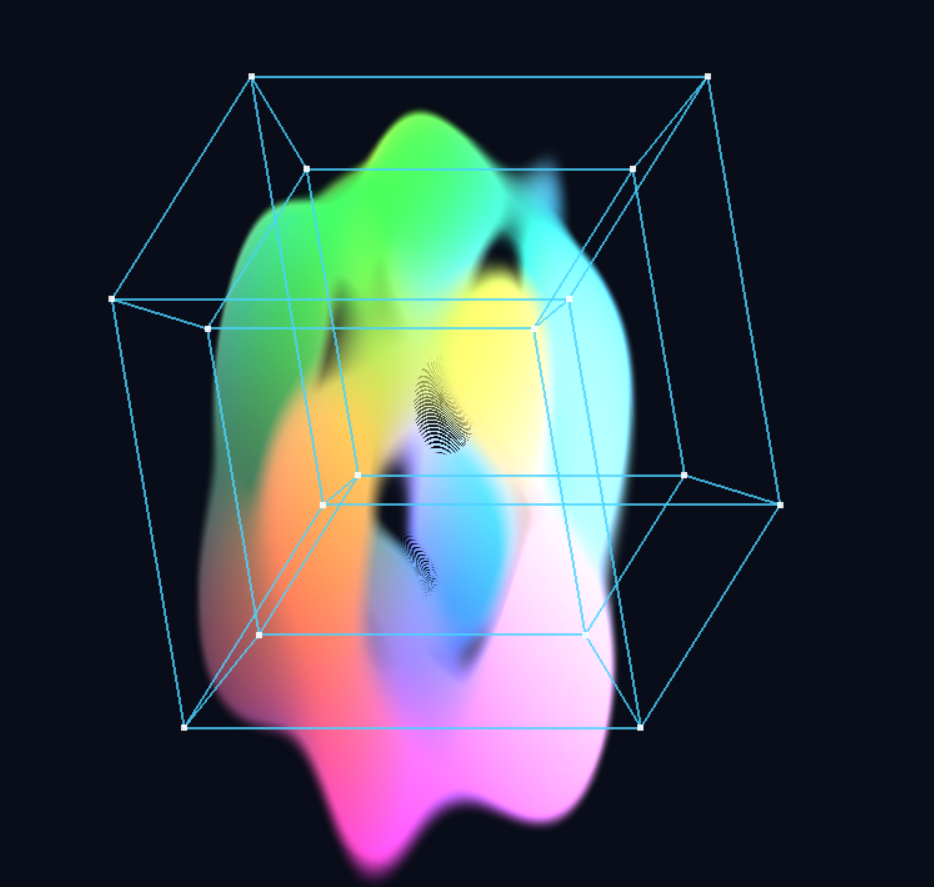
Arbitrary slice navigation: the viewing hyperplane rotates continuously through 5D, revealing structure that axis-aligned slices would miss.
From Discrete to Continuous Navigation
# Orthogonal slice: pick 3 axes from {x,y,z,w,t}
view_axes = [0, 1, 2]  # XYZ slice at fixed W, T

# Arbitrary slice: define 3D hyperplane by basis vectors
basis_1 = normalize([1, 0, 0.3, 0.1, 0])   # Not axis-aligned
basis_2 = normalize([0, 1, -0.2, 0, 0.1])
basis_3 = normalize(cross_5d(basis_1, basis_2, ...))

# Slice coordinates become linear combinations
point_5d = origin + u*basis_1 + v*basis_2 + w*basis_3
Smooth interpolation between different "views" of the 5D structure becomes possible—the slice plane itself can be animated, creating trajectories through the space of all possible 3D cross-sections.
Two 5D Fields: (x,y,z,w,t) ↔ (x,y,z,θ,φ)
The Key Observation
We start with a procedural field defined over five dimensions. But when we view a 3D slice, the viewing direction itself adds two more degrees of freedom. This gives us another 5D field—structured differently, but parallel in form:
Original Field
(x, y, z, w, t) → RGBAw, t are latent/temporal axes. We pick values for them, then explore the resulting 3D structure.
View-Based Field
(x, y, z, θ, φ) → RGBAθ, φ are viewing angles. We pick a viewpoint, then see the resulting 3D appearance.
Both are 5D → appearance mappings. The interpretation differs—the original field's extra dimensions encode latent/temporal state, while the view field's encode observer perspective—but the mathematical structure is identical. This is the foundation for the feedback loop.
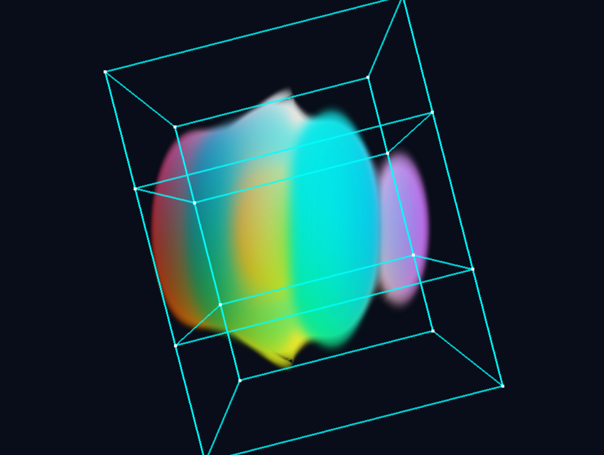
View from angle (θ₁, φ₁)
View from angle (θ₂, φ₂)
Fixing (w,t) and varying (θ,φ) produces training data for a NeRF—which encodes the same structure, but parameterized by viewing angle instead of latent coordinates.
Two Complementary Feedback Loops
Different Domains, Complementary Roles
The key insight: these two loops operate on different domains and serve complementary purposes. Understanding this distinction is crucial.
Loop 1: NeRF Iteration (Function → Function)
This loop evolves the background field itself. Starting from the purely procedural field (which is just a function—no stored values), we render views and train a NeRF to encode this field in a new parameterization.
# Iteration 0: Start with procedural field
procedural: (x,y,z,w,t) → RGBA     # Pure function, no stored data

# Fix (w,t), render many views
views = [render_procedural(w₀, t₀, θ, φ) for θ, φ in viewpoints]

# Train NeRF to encode this view-field
nerf_1: (x,y,z,θ,φ) → RGBA         # NeRF encodes the field

# Reinterpret: treat (θ,φ) as new (w,t)
# Now nerf_1 can be queried as a new background field!

# Iteration 1+: NeRF → NeRF
views = [render_nerf(nerf_1, w₀, t₀, θ, φ) for θ, φ in viewpoints]
nerf_2 = train_nerf(views)
# ... and so on
After the first iteration, it's NeRF → NeRF all the way down. Each cycle produces a new neural encoding of the transformed field. The background field evolves through representation change.
Loop 2: Taichi Diffusion (Numerical Evolution ON the Field)
This loop operates on top of whatever background field currently exists (procedural or NeRF). It samples a 3D slice, runs reaction-diffusion dynamics, and tracks the deviation.
# Taichi operates on the current background field
background = current_field  # Could be procedural OR nerf_n

# Sample a 3D slice at fixed (w,t)
slice = sample(background, w=w₀, t=t₀)

# Run diffusion dynamics
state = initialize_from(slice)
for step in range(n_steps):
    state = diffusion_step(state, slice)  # BG modulates dynamics

# Track what evolved
deviation = state - slice  # This is the "foreground" structure
This is local, numerical evolution—patterns emerge and evolve on the current background, whatever that background happens to be.
Why Both?
The loops complement each other:
- NeRF loop: Evolves the background field itself (global transformation)
- Taichi loop: Evolves structure on the background (local dynamics)
You could run Taichi on a procedural background, or on a NeRF-encoded background, or alternate between them. The NeRF loop changes what you're evolving on; the Taichi loop changes what's happening on it.
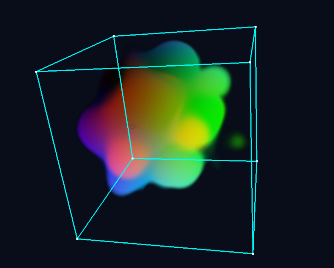
The NeRF feedback loop: field → views → train NeRF → NeRF encodes new field → repeat
The Blending Problem
What does it mean to "blend" two NeRFs or interpolate between fields? Unlike blending two images (just mix pixel values), these are generators—functions that produce values on demand. To blend them, you must keep both in memory.
# Naive blending: query both, interpolate outputs
def blended_field(x, y, z, w, t, alpha):
    val_a = nerf_a(x, y, z, w, t)   # Need nerf_a in memory
    val_b = nerf_b(x, y, z, w, t)   # Need nerf_b in memory
    return (1-alpha) * val_a + alpha * val_b

# After N iterations: N networks in memory!
# Rendering slows down linearly with iteration count
This is a fundamental tension: smooth evolution via blending requires keeping history, but history accumulates. After 100 iterations, you'd need 100 NeRF networks.
Potential Solutions
Several directions might address this:
- NeRF Distillation: Train a single "student" NeRF to approximate the blended output of multiple "teacher" NeRFs, then discard the teachers.
- NeRF Merging Research: Recent work explores combining multiple NeRFs into unified representations—could enable "committing" a blend to a single network.
- Lazy Evaluation: Only materialize the blend when needed, accepting the computational cost during rendering.
This connects to a broader theme in the Symbolic Math project: the tension between symbolic/lazy representations (compact but expensive to evaluate) and materialized/eager ones (fast but memory-heavy). The NeRF iteration faces the same tradeoff.
Taichi: Not Limited to 3D
The examples show Taichi operating on 3D slices, but this is a practical choice, not a fundamental limitation. Reaction-diffusion dynamics work in any dimension—you could run them on a 4D or 5D tensor directly.
# 3D slice (current implementation)
slice_3d = sample_field(w=w₀, t=t₀)  # Shape: (Nx, Ny, Nz)
evolved_3d = run_diffusion(slice_3d)

# 4D slice (fix only t)
slice_4d = sample_field(t=t₀)        # Shape: (Nx, Ny, Nz, Nw)
evolved_4d = run_diffusion(slice_4d)

# Full 5D (no slicing)
full_5d = sample_field()             # Shape: (Nx, Ny, Nz, Nw, Nt)
evolved_5d = run_diffusion(full_5d)  # Memory-intensive!
The constraint is memory: a 256³ volume is ~16M voxels; a 256⁵ volume would be ~1 trillion. But for modest resolutions or sparse representations, higher-dimensional diffusion is entirely feasible.
The Experimental Nature
This project is purely exploratory. There's no theorem guaranteeing convergence, no proof that interesting structure will emerge. The questions are empirical:
- "What does this iteration look like after 10 cycles? 100?"
- "Does blending old and new fields produce smoother evolution?"
- "Can we guide the process toward particular structures?"
- "What happens if we combine both loops—diffusion AND representation cycling?"
The goal isn't to prove something works—it's to discover what's interesting before deciding what's useful.
Future Directions
Current Limitations
The project is theoretically interesting but visually less compelling than hoped. Some aspects are unnecessarily complex in the current implementation:
- The highly symmetric procedural fields produce results that aren't substantially different from using tabulated data.
- We could simplify by pre-computing a finite 5D tensor at startup and applying periodic boundary conditions (wrapping around on all axes). This would eliminate the need to maintain analytical field definitions.
Simplifying the Pipeline
If we start with a numerical 5D field (tabulated tensor), the NeRF iteration becomes more uniform: each cycle performs dense sampling to convert the NeRF encoding back into a numerical field, which then feeds the next iteration.
# Numerical-first pipeline
tensor_5d = precompute_field()           # Dense 5D tensor at startup

# NeRF iteration cycle
views = render_from_tensor(tensor_5d, viewpoints)
nerf = train_nerf(views)
tensor_5d = dense_sample(nerf)           # Back to numerical
# Repeat...
This avoids the complexity of maintaining both analytical field definitions and NeRF networks simultaneously. The tradeoff is memory (tabulated fields are larger), but the pipeline is conceptually cleaner.
Where It Gets Interesting
The framework becomes more meaningful with less symmetric, aperiodic fields:
- Non-periodic procedural functions where the structure genuinely varies across the full 5D domain—here, infinite evaluation matters.
- Data-driven fields (e.g., volumetric captures, simulations) where the 5D structure comes from real phenomena rather than mathematical formulas.
- Hybrid approaches: procedural base with learned refinements that break symmetry.
The NeRF iteration machinery is overkill for symmetric fields but could reveal genuinely novel structures when applied to richer, less predictable data.
Dimension Mapping (Original System)
The base visualization assigns five dimensions to different roles:
Spatial Axes
3D view space
Latent Dimension
Navigate via slider
Time
Animates the view
Any permutation is valid—smoothness in 5D implies coherent structure from any projection. Swapping which axis serves as time versus latent dimension produces completely different animations from the same underlying field.
NeRF Input Space: (x, y, z, θ, φ)
A Neural Radiance Field takes a different 5D input: spatial position (x, y, z) plus viewing direction (θ, φ). The network outputs color and density for that point as seen from that angle.
Spatial Position
Point in 3D scene
View Direction
Spherical angles
The Equivalence
Both systems map 5D → RGBA. If we have a NeRF trained on arbitrary viewpoints, we can reinterpret it as a time-varying volumetric field: treat one angular dimension as time (θ → t), and the other as a latent axis (φ → w). The network becomes a procedural 5D field—exactly the structure we started with.
# NeRF interpretation
nerf(x, y, z, θ, φ) → RGBA

# Reinterpret as time volume
volume(x, y, z, w=φ, t=θ) → RGBA

# Same function, different semantics
Mathematical Foundation
5D Distance Metric
The fractal is computed using the 5D Euclidean distance:
d = √(x₀² + x₁² + x₂² + x₃² + x₄²)Iterative Formula
A 5D Mandelbrot-style fractal uses:
z_{n+1} = f(z_n) + cwhere z and c are 5-dimensional vectors, and f represents the fractal transformation (often a power operation extended to 5D using geometric algebra or quaternion-like structures).
Projection to 3D
Given dimension assignment (i, j, k, w, t), the 3D point displayed is:
x_3D = dimensions[i]
y_3D = dimensions[j]
z_3D = dimensions[k]

// Fix hidden dimension w at slider value
dimensions[w] = w_value

// Animate time dimension t
dimensions[t] = sin(time * frequency)
Projection Mathematics: Intuition
What is a Projection?
A projection is a way of "squashing" higher-dimensional space into lower dimensions. Think of a 3D object casting a 2D shadow - you lose depth information, but retain shape.
For a 5D point p = (p₀, p₁, p₂, p₃, p₄), projecting to 3D means:
// Choose 3 dimensions to display
Projection(p) = (p_i, p_j, p_k)

// The other dimensions (p_w, p_t) are "collapsed"
Orthogonal vs. Perspective Projection
This viewer uses orthogonal projection - parallel lines in 5D remain parallel in the 3D view. The alternative, perspective projection, would make distant 5D points appear smaller, but is harder to interpret for higher dimensions.
Orthogonal:    (x,y,z,w,t) → (x,y,z)  [simply drop w,t]
Perspective:   (x,y,z,w,t) → (x,y,z)/f(w,t)  [scale by distance]
The Hidden Dimension Slice
When you set the hidden dimension w to a value w₀, you're looking at a 3D slice (technically a 4D slice with time) of the 5D fractal:
Slice at w = w₀:
S = {(x,y,z,w₀,t) : fractal(x,y,z,w₀,t) < threshold}

This is a 4D manifold embedded in 5D space
As you move the slider through different w values, you're traveling through the 5D structure perpendicular to your viewing plane. Each position shows a different cross-section.
Continuity and Smoothness
Why Smooth in 5D Means Smooth in Any View
Here's the key insight: smoothness is an intrinsic property of the 5D fractal, independent of how you view it.
Mathematically, a function f: ℝ⁵ → ℝ is smooth if all its partial derivatives exist and are continuous:
∂f/∂x₀, ∂f/∂x₁, ∂f/∂x₂, ∂f/∂x₃, ∂f/∂x₄ all continuous
∂²f/∂x_i∂x_j all continuous
... and so on
When you project to 3D, you're looking at a restriction of this smooth function:
// Original 5D function
f(x₀, x₁, x₂, x₃, x₄)

// Projected 3D view (fixing x₃=w₀, x₄=t₀)
g(x₀, x₁, x₂) = f(x₀, x₁, x₂, w₀, t₀)
If f was smooth in 5D, then g is automatically smooth in 3D because:
∂g/∂x₀ = ∂f/∂x₀ (just restrict the derivative)Continuity is preserved under projection. No matter which 4 dimensions you choose to view, the projection inherits the continuity of the original 5D structure.
Smooth Transitions Between Views
When you switch which dimensions map to XYZ, the fractal structure morphs smoothly because you're continuously rotating your viewpoint in 5D space. Think of it like walking around a 3D sculpture - the object doesn't change, only your perspective does.
The transition can be interpolated:
// Old view: dimensions (0,1,2) → XYZ
// New view: dimensions (1,2,3) → XYZ

// Interpolate with rotation matrix R(θ) in 5D
view(θ) = R(θ) · original_view

As θ: 0 → π/2, smoothly rotate from old to new
Coherence Across All Projections
The "coherence" you see - that the fractal looks structured from any angle - comes from the fact that fractals have self-similarity in all directions. The 5D fractal has correlation between all its dimensions:
// A point is in the fractal set if:
|z_n| < threshold for all n iterations

where z_n ∈ ℝ⁵ evolves via:
z_{n+1} = f(z_n) + c

This evolution couples ALL 5 dimensions together
Because the dimensions are coupled through the iterative formula, structure in one dimension influences structure in all others. You can't have chaos in one view and smoothness in another - the 5D dynamics enforce global coherence.
Mathematical Guarantee
For Mandelbrot-type fractals, the boundary (where |z_n| ≈ threshold) is a 4D manifold embedded in 5D space. This manifold is closed and bounded (compact), which guarantees:
- Any projection to 3D is bounded (won't extend to infinity)
- Any projection to 3D is continuous (no sudden jumps)
- Topological features (holes, connectedness) are preserved in generic projections
This is why switching views doesn't break the fractal - you're always looking at different slices of the same underlying 4D boundary surface.
Future Directions
Open Questions
- Convergence: Does the procedural → NeRF → reinterpret cycle converge to stable structure?
- Attraction: Can we introduce forces that pull representations toward similarity under projection?
- Hybrid dynamics: What happens when diffusion and neural resampling operate simultaneously?
- Topological persistence: Which features survive multiple representation changes?
Technical Implementation
GPU Acceleration
The system uses Taichi for GPU-accelerated simulation (diffusion dynamics on 128³–256³ grids) and custom GLSL shaders for real-time ray marching. Memory management is critical—a 256³ single-channel field requires 64MB, three-channel requires 192MB.
Performance Targets
- Simulation: 10–20ms per frame for diffusion updates
- Rendering: 16–33ms per frame for ray marching
- Combined: 30 FPS with simulation + rendering