Drawing with harmonics
Draw a gesture, keep its timing, and inspect its moving spectrum. Compare local STFT, global Fourier coefficient selection, cosine symmetry, pinned-end sine modes and local wavelet detail—with a working reconstruction for each.
Explore connections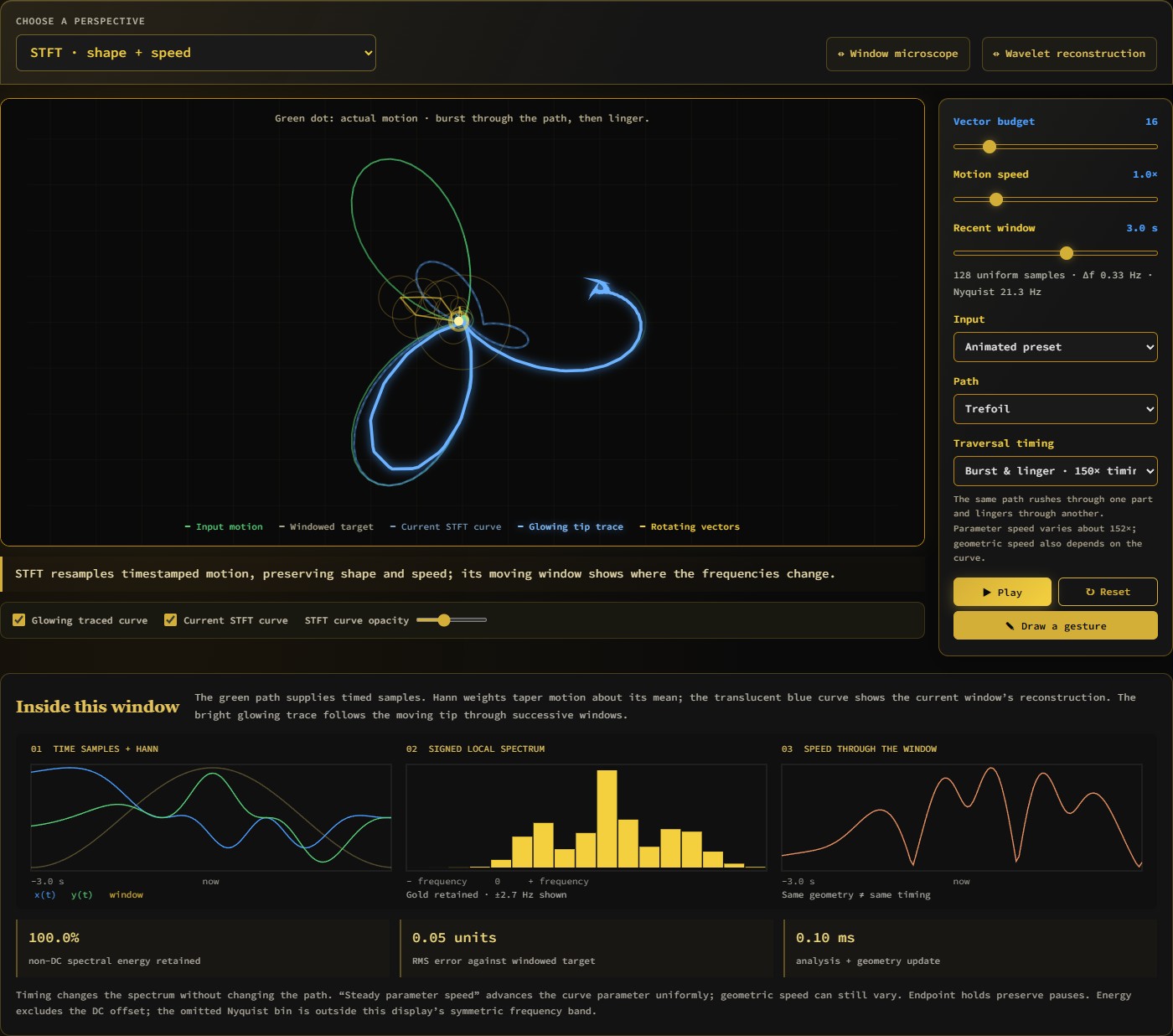
Open the application, then follow what changes
A drawing is a timed performance, not only an outline. Keep a gesture's changing speed and inspect its moving STFT spectrum, then compare global Fourier selection, cosine symmetry, pinned-end sine modes and local wavelet detail through their reconstructions.
-
01
Capture the gesture
Draw a path while retaining when and how quickly it was drawn.
-
02
Choose a decomposition
Compare local windows, global harmonics and alternative boundary conventions.
-
03
Inspect the coefficients
Reveal moving spectral energy or the local detail being retained.
-
04
Reconstruct the motion
Watch the selected components recover the path and its timing.
A drawing is also a performance
A familiar Fourier drawing turns a contour into rotating vectors. This workbench asks what happens when the timing matters too: trace the same shape slowly, rush through one part, or hold still. The shape can be unchanged while its local spectrum changes. A trefoil runs immediately so this difference is visible before drawing anything.
STFT exposes recent motion; global Fourier exposes an entire gesture. The same default trefoil rushes and lingers, so its uniform time samples record a changing speed. Cosine and pinned-end sine modes change the boundary assumptions; Haar wavelets isolate local detail.
Keep the shape and the speed
Timestamped motion is interpolated onto evenly spaced time samples, preserving pauses and changes of speed. Windowed sketch tapers displacement toward its mean with a Hann window; adding more sketch vectors reproduces that tapered target, rather than undoing the taper.
Choose STFT reconstruction → Match sampled path in the live studio. Inverse STFT combines overlapping Hann-windowed frames, retaining all bins including Nyquist, and normalizes their accumulated weights. The blue curve recovers all 128 recent time samples; the gold tip follows the latest recovered sample.
The match is exact to floating-point accuracy at those interpolated samples, not at unknown points between mouse events. The latest sample is one interval behind the pointer—about 23 ms with the default three-second window—and the interface reports that delay alongside reconstruction error.
Change the extension, change the motion
The periodic Fourier mode treats a sampled drawing as z[n] = x[n] + i y[n]. Each coefficient contributes a rotating vector, with radius set by amplitude and angle set by frequency and phase. Keeping fewer components reveals which motion they carry. Contiguous frequencies and automatically selected largest coefficients are two selection policies within this same Fourier basis. Compare their errors using the same number of vectors.
A scalar cosine and a scalar sine both oscillate along a fixed direction; the complex exponential is the rotating object. The cosine view appends a reversed copy and draws equivalent counter-rotating pairs, so the gesture goes out and back. The sine view draws combined fixed-axis contributions after subtracting a straight endpoint baseline, then restores that baseline. Neither extension requires a mirror-symmetric drawing.
Fast enough to inspect while drawing
The live window uses a radix-2 FFT with cached trigonometric factors and reusable working arrays. Its retained reconstruction is cached between analysis updates, and input trails are batched for drawing. Animation and analysis therefore have separate work budgets.
Numerical tests compare FFT coefficients against independent direct sums, and check inverse STFT on endpoint impulses, short buffers, different overlaps and stationary holds. Responsiveness and reconstruction accuracy are measured separately.
A longer look resolves frequencies—and smears events
Compare two FFT spectrograms of exactly the same signal: two nearby tones, a brief burst or a changing pitch. A long window separates close frequencies while a short window localizes the burst. More display pixels alone cannot recover information excluded by the observation window.
Rebuild a path from local details
Haar wavelets replace global oscillations with a hierarchy of averages and differences. Recover the timed path one scale at a time, inspect the coefficients, and compare reconstruction error. Changing one detail affects its local time interval; a Fourier component extends across the whole recording.
The piecewise-constant reconstruction makes Haar’s support explicit. With all coefficients retained, the inverse recovers the sampled x/y signals; reducing the scale budget deliberately loses detail. This is a working multiresolution transform, with perfect reconstruction and energy tests.
From drawn motion to physical vibration
A pinned uniform spring chain has discrete sine-shaped eigenmodes. The sine reconstruction here uses that basis to represent a gesture after subtracting its endpoint baseline. You can see how adding modes rebuilds local shape while the endpoints stay fixed.
Modal2D takes the modal idea into a physical object: geometry, material and supports determine the finite-element eigenmodes, then excitation and damping determine its sound. This is a connection through basis decomposition; arbitrary instrument modes are not assumed to be Fourier sinusoids.
More recorded views · 3
Current scope
- Dominant Fourier components selects amplitude-ranked Fourier coefficients; it is not empirical mode decomposition or a Hilbert–Huang transform.
- Finite samples, the chosen extension and the retained frequencies define the reconstructed curve. Full inverse STFT recovers the 128 resampled points to floating-point accuracy, with one sample interval of delay; it does not recover unrecorded continuous detail. The microscope uses synthetic signals to isolate window length.