Desktop application Research
Interactive Video

RadianceLab

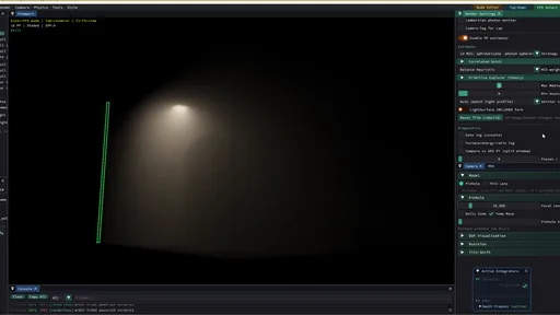
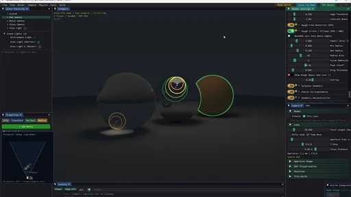
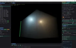
An interactive CPU/GPU renderer for exploring light transport in a variety of scenes. Switch among ten selectable modes spanning established methods and photon estimators from my own research, edit materials and media in place, inspect paths and intermediate structures, then set up the camera and refine a beauty shot.

Explore connections Brochure · 39 chapters ↓
Scenes → transport → inspection
AuthorRenderInspect
Technical docs · native implementation Go one layer deeper: surface curves, mesh sheets, projector imaging, cameras and the backend support matrix.Validation · images, timings & checks Inspect retained native renders, estimator comparisons and the limits of the measurements.
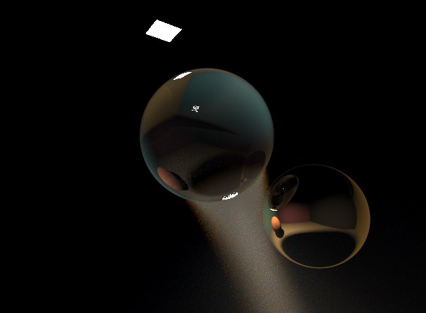
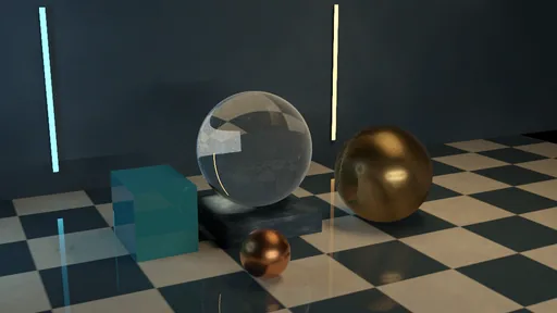
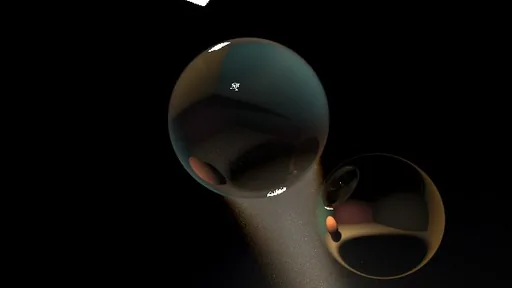
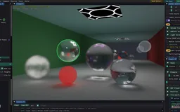
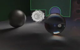
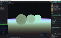
Photon-hourglass rendering: refractive transport through a glass sphere forms a concentrated caustic in a participating medium, beside a reflective gilt sphere.
An implemented pipeline

Work through the viewfinder, then refine the image

Composition, scene editing, transport inspection and final rendering share the same workspace. The goal is to make research methods usable while their internal operation stays visible.

  1. 01

    Compose and explore

    Place geometry, emitters and media; move through the scene in first person and choose a subject.

  2. 02

    Author what the scene shows

    Edit material and medium nodes, inspect their previews, and apply the graph to the working scene.

  3. 03

    Choose and inspect transport

    Switch among rendering modes; reveal paths, photons, guiding fields and the active image producer.

  4. 04

    Frame the photograph

    Set focus and aperture, adjust perspective with dolly zoom, and use projection or UV baking when authoring calls for it.

  5. 05

    Refine and preserve

    Hold the view for progressive accumulation, compose its display treatment, then preserve images and settings through the supported export routes.

Breadth · Methods

Established transport in one workspace

PT, LT, BDPT, photon mapping, connection/merging, primary-space Metropolis and guiding sit beside partial and research branches in a ten-mode studio.

Breadth · Image formation

Color, media and measurement

RGB and wavelength-sampled tracing, rich surface and emission models, participating media, reservoir reuse and ToF broaden what the renderer can study.

Breadth · Workflow

A visual instrument for scene work

Node previews, first-person camera work, lens controls, projection, UV baking, intermediate inspection and post-processing connect setup to the final image.

Original research

Extend the photon into geometry

The most complete implementation of the photon-primitive framework I am aware of: a broad family of swept primitives, compatible MIS strategies, and refracted hourglass sheets for difficult light paths.

Capabilities / connected systems

Read the system by what it makes possible

Related techniques belong to one family. Follow a family into the interface, recorded results and mathematical detail.

01 / 08

Photon hourglass: sharp volumetric caustics through glass

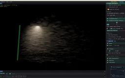
An analytic photon primitive draws the light refracted through a glass sphere as a whole sheet, sharp within a second of holding the camera still; traced mesh sheets carry the idea to triangles, with a biased preview for walking.

The refracted hourglassSharp within a secondChains and off-axis followersMesh photon sheetsFast structure previewThe tridirectional hourglass
Feature set · 6 capabilities
  • The refracted hourglassRotational symmetry sweeps a two-interface Snell chain into a caustic sheet, with an index-one limit and an independently checked crossing solve.
  • Sharp within a secondKernel-free sheets at 1.2 to 1.5 ms a pass for one ball on laptop CPU cores, 35 to 48 times lower variance than photon beams at equal time on a two-ball chain; paired with an ordinary estimator, the easy direct light still converges last.
  • Chains and off-axis followersCollinear chains keep the analytic solve through every ball; a follower moved off the axis needs a numerical crossing search and a fresh primitive per sample.
  • Mesh photon sheetsFinite fans of traced rays through closed triangle meshes, so Suzanne, a teapot and a torus cast hourglass caustics too.
  • Fast structure previewA rasterized, biased viewfinder that keeps the sheets smooth while the camera moves.
  • The tridirectional hourglassGlass-seeded hourglass members, shown for completeness beside the light-seeded strategy 20 that outperforms them; the reflection cone is their one positive result.
02 / 08

Original research: photon-primitive extensions

Extend sampled photons into beams, rings, surfaces and refracted hourglass sheets, carrying their geometry, measure and supported paths through the estimator.

A dimensional familyGeneralized connectionsPhoton primitivesCorrelated primitive poolsConservative reuse
Feature set · 5 capabilities
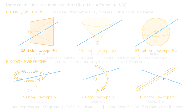
  • A dimensional familyPoints, beams, rings, arcs, spheres, planes and cones reveal which direction, distance or source coordinates remain sampled.
  • Generalized connectionsA camera ray queries a swept locus; projected Jacobians and all admissible roots convert geometry into an estimator.
  • Photon primitivesHand-pick the swept dimensions to get a technique with MIS: 34 strategy slots, stacked so every transport has exactly one owner.
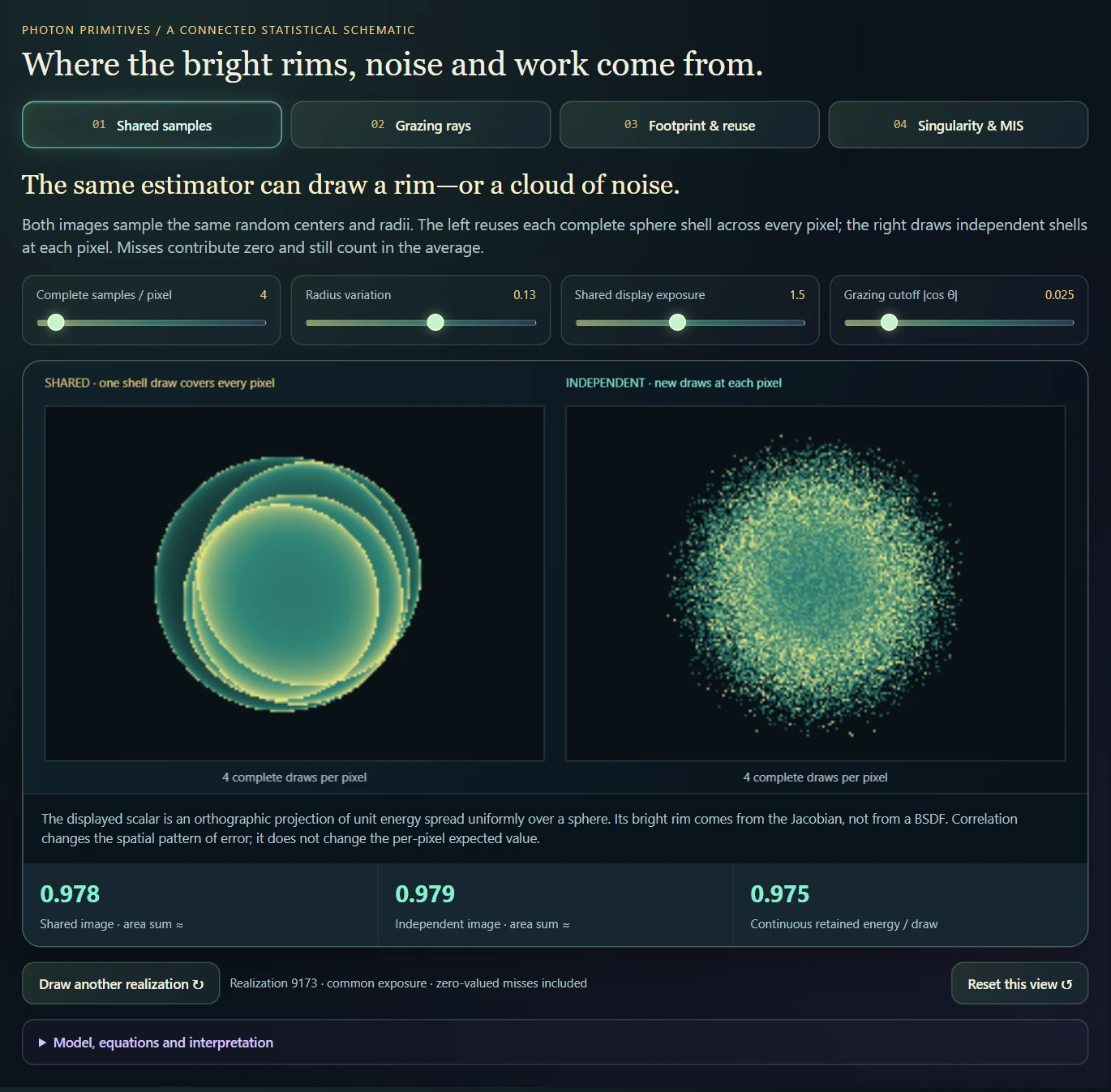
  • Correlated primitive poolsShared samples preserve the intended marginal estimate while changing spatial covariance and making geometric footprints visible.
  • Conservative reuseDistinguish repeated seed reconstruction, cached primitive records and bounded CPU gathering; compare equal-work cost separately from image error.
03 / 08

Transport methods, cluster by cluster

Nine of the ten selectable modes, grouped by how they find light paths: tracers, photon maps, connection and merging, Metropolis chains, learned or specular-aware proposals for hard paths, and rasterization; the photon-primitive mode has its own families above. Each chapter states what runs, where it fails and why.

Path tracer, light tracer and BDPTPhoton mapping and progressive photon mappingVCM and UPBPMLT and PSSMLTPath guiding and manifold explorationRasterization
Feature set · 6 capabilities
  • Path tracer, light tracer and BDPTSeven light strategies from one GPU compute shader, with examples of their successes and failures. The BDPT strategy pyramid stays interactive while you walk—a workflow I have not found in another interactive BDPT project.
  • Photon mapping and progressive photon mappingFast, biased density estimation with per-batch radii that shrink as passes accumulate.
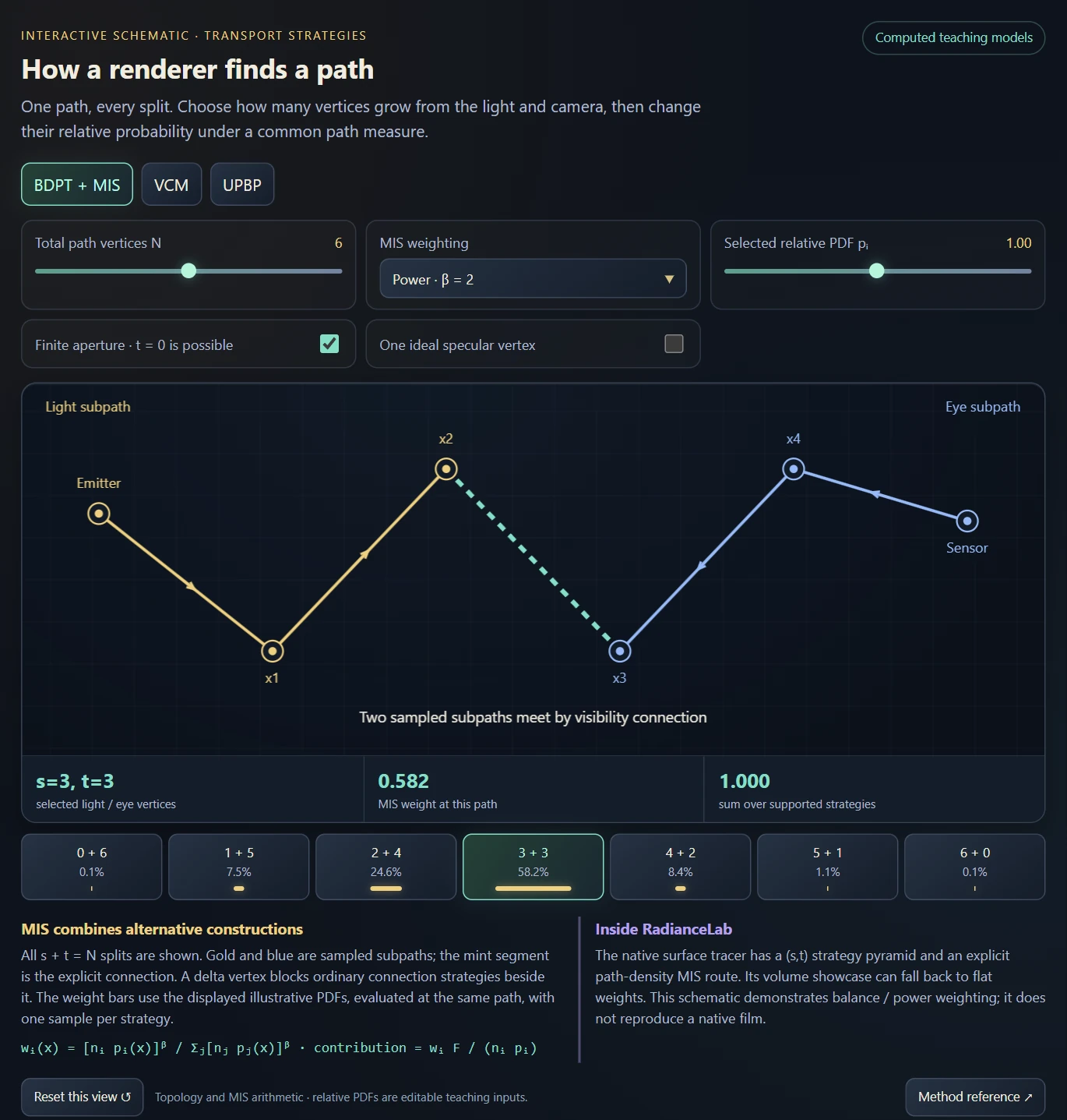
  • VCM and UPBPConnection and merging on surfaces, and an audited subset of Unifying Points, Beams, and Paths in media.
  • MLT and PSSMLTPrimary-sample Markov chains with large and small steps, rollback and chain statistics.
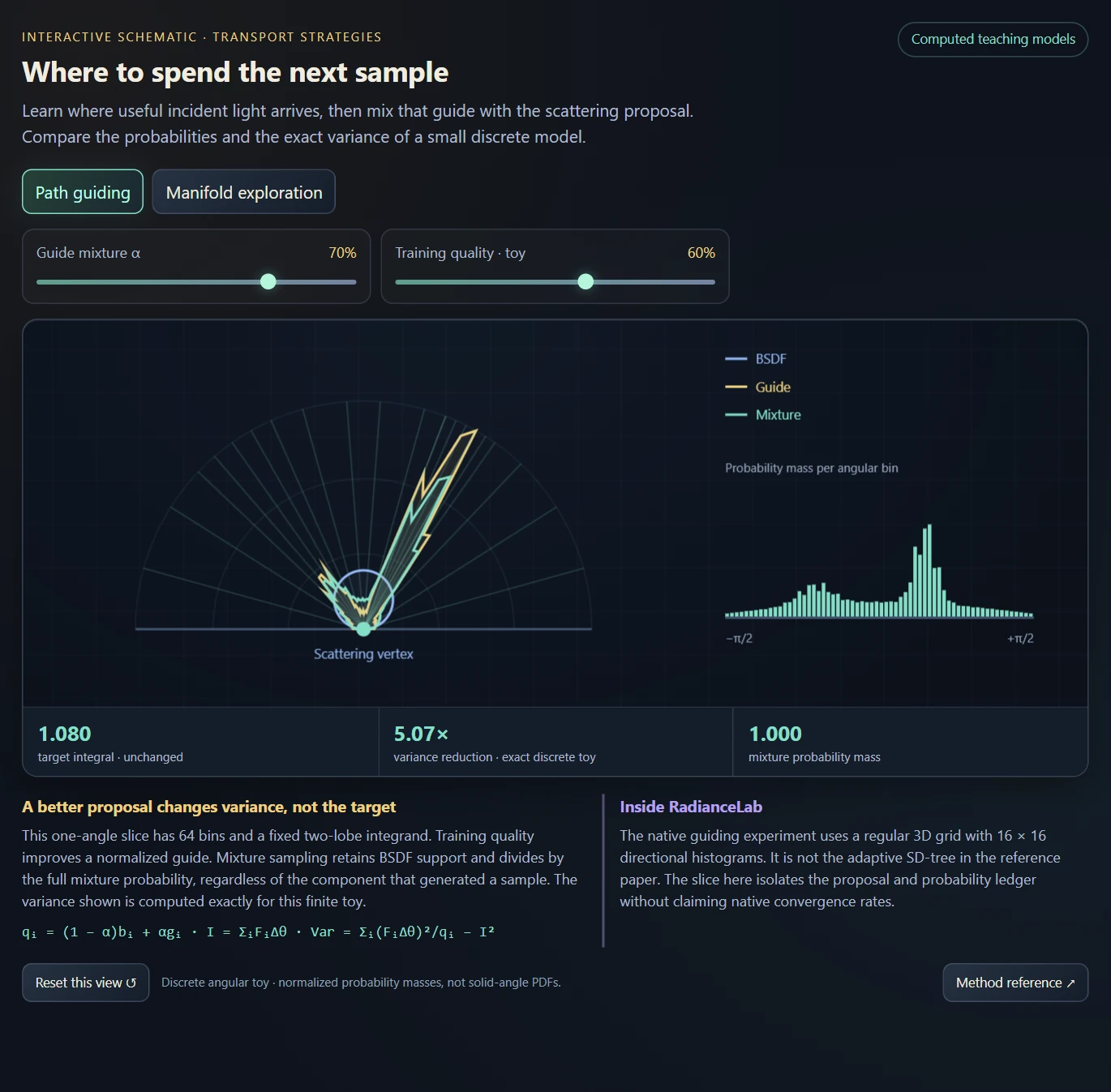
  • Path guiding and manifold explorationTwo mechanisms for hard paths, a learned directional proposal and specular-aware mutations, with interactive schematics.
  • RasterizationThe fastest route, plus two ways to composite traced appearance into the raster image.
04 / 08

Explain noise before trying to remove it

Inspect contribution tails, combine complementary geometric proposals and check each estimator against the quantity it is meant to estimate.

Common-measure MISAcceptance and contribution tailsCustom primitive combinationsControlled emitter experimentsControlled numerical evidence
Feature set · 5 capabilities
  • Common-measure MISCompatible alternatives compare their real event densities and support; finite-radius members retain an explicit consistency qualification.
  • Acceptance and contribution tailsMiss probability, conditional weights and fold singularities explain why one variance number can conceal different problems.
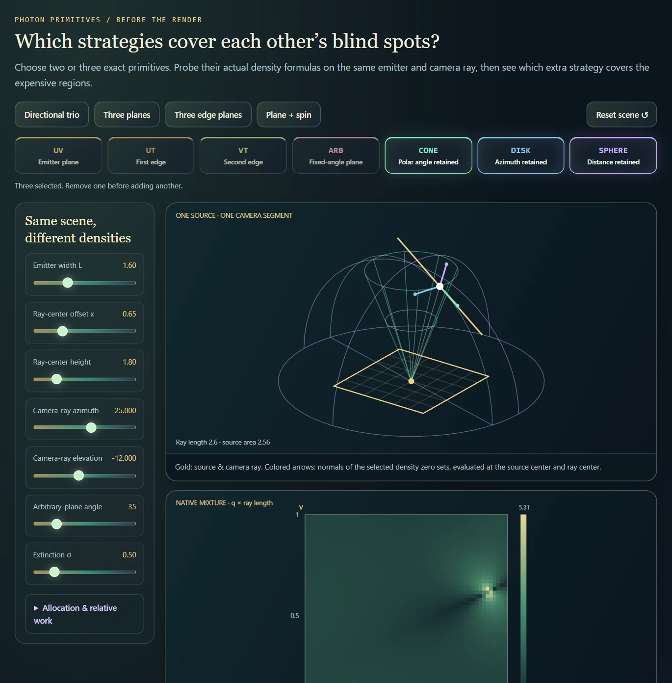
  • Custom primitive combinationsCompare any selected pair or trio, inspect shared density zeros, and distinguish exact-family MIS from finite-radius hybrid blends.
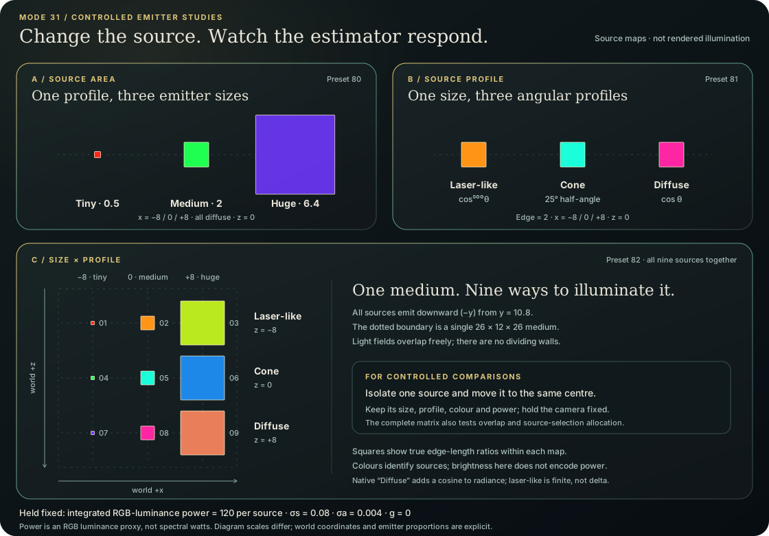
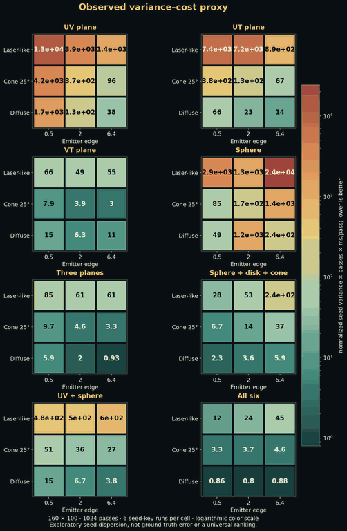
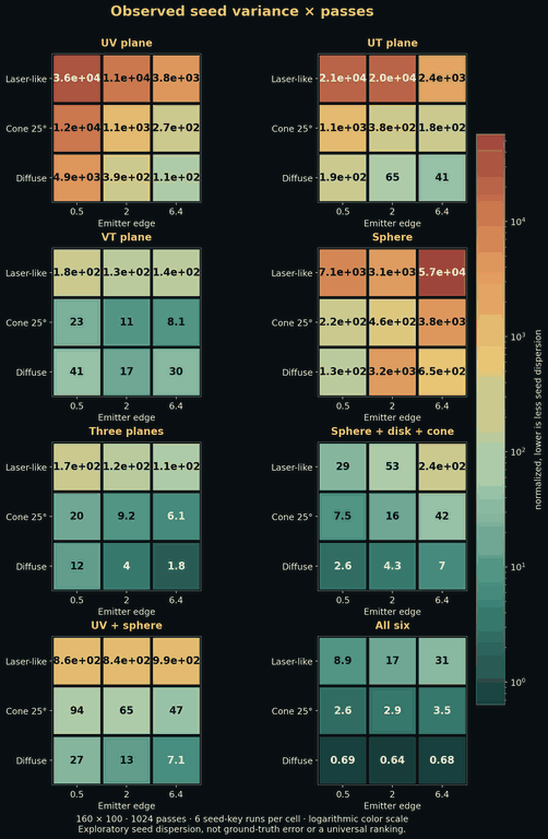
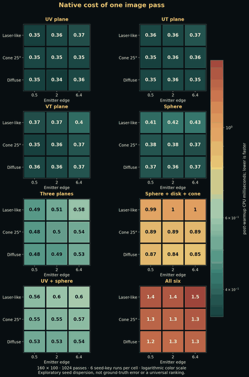
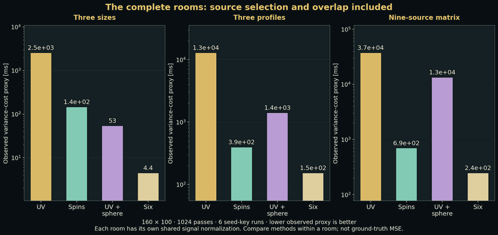
  • Controlled emitter experimentsThree colored medium-box scenes and a centered 3 × 3 size/profile study connect native renders to repeated-film noise and measured CPU cost.
  • Controlled numerical evidenceFinite differences, limiting cases, same-draw replays and linear-film exports separate numerical correctness from visual plausibility.
05 / 08

Breadth of image formation: color, materials, media and optical measurement

RGB and spectral color, surfaces, sources, participating media and reservoir reuse define what a scene can express; CPU modes implement narrower, stated subsets. Projectors, path-length gates and time of flight turn the same scene into a measurement.

RGB and wavelength-sampled transportMaterials, media and emissionReservoir reuse and temporal toolsProjector and path-length gatesFour-bucket time of flight
Feature set · 5 capabilities
  • RGB and wavelength-sampled transportOne sampled wavelength per path, Gaussian-lobe spectra for surfaces and light sources, and a Cauchy index shared with the photon hourglass.
  • Materials, media and emissionBSDFs, textured and procedural inputs, spatial absorption/scattering and source profiles define the available scene models; a medium graph runs as constants, a recognized live procedure or a baked volume.
  • Reservoir reuse and temporal toolsDirect-light candidate reservoirs reuse information spatially and temporally; a separate screen-space indirect route is labeled experimental.
  • Projector and path-length gatesModulated illumination and selected arrival lengths turn transport into an observable signal rather than a display overlay.
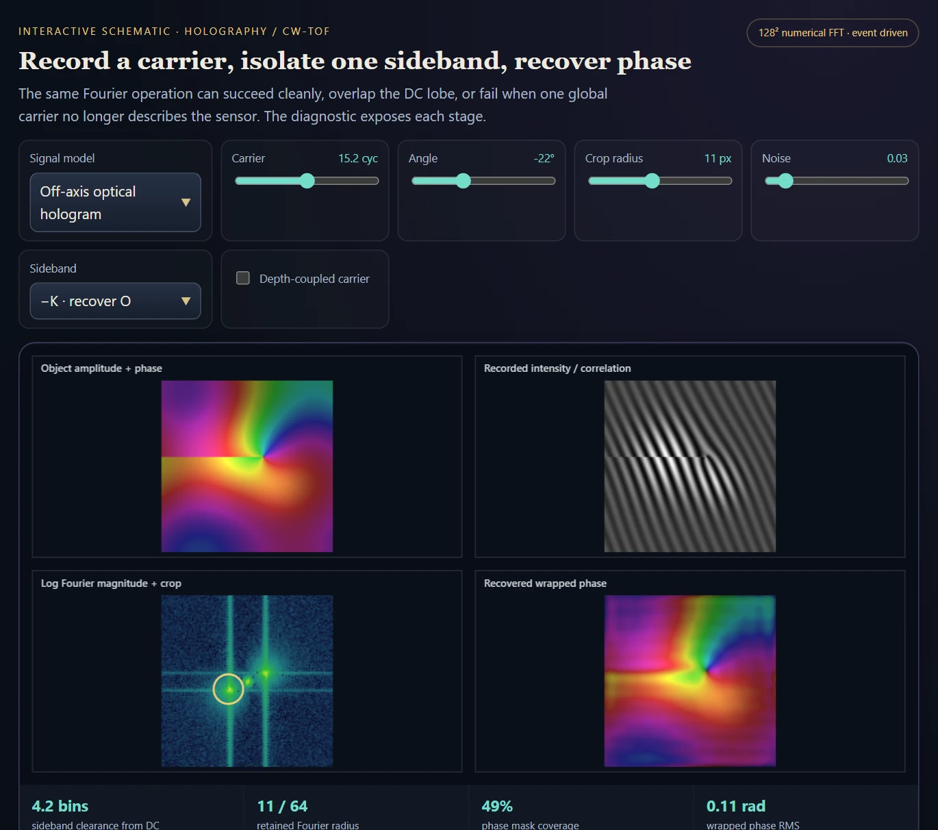
  • Four-bucket time of flightRecover phase and amplitude while distinguishing wrapping, multipath, synthetic-depth controls and assisted reconstruction.
06 / 08

Walk in, edit, render and inspect

Walk through the scene, change what is visible, switch the rendering technique under a live preview, take a high-quality photograph, and draw the auxiliary structures and intermediate results behind the film.

First-person viewfinderA physical camera and moreEdit in placeLive technique switchingTake a shotEvery intermediate on screen
Feature set · 6 capabilities
  • First-person viewfinderWalk with WASD or fly in noclip, select by click or crosshair, and keep the active film refreshing while the camera moves.
  • A physical camera and morePinhole, thin-lens and tilt/shift models, shared aperture shapes, dolly zoom, focus aids, a depth-reprojected photograph and a hologram record-and-replay tool.
  • Edit in placeA transform gizmo, per-object BSDF, emission and medium components, spectral curves and typed node graphs edited beside the render.
  • Live technique switchingTen modes on number keys, a deferred switch with automatic enable, an active-producer thumbnail and labeled biased previews; each mode keeps its own film and invalidation.
  • Take a shotChosen output size and pass budget, still or moving-camera exposures, PNG plus linear HDR/PFM and a JSON record, then back to the preview.
  • Every intermediate on screenRay tree, photon clouds and KD-trees, connections and merges, mutation traces, guiding arrows, the BDPT pyramid, the missing-transport fill and photon-primitive instruments.
07 / 08

Smaller features: baking, post-processing, NPR and a CV toolbox

Bake a projected image into a material, compose the final image with post-processing and NPR, and read the rendered view with a small computer-vision toolbox.

Projection and UV bakingNPR and effectsCV toolbox
Feature set · 3 capabilities
  • Projection and UV bakingCarry an imported image or clean-frame capture through camera coordinates into a baked material or a live surface projection.
  • NPR and effectsTwenty-one NPR modes and a bank of 157 toggleable image operators on the live scene; history-dependent and field effects keep their own implementation notes.
  • CV toolboxPoint-cloud reconstruction from depth and normals, a bilateral grid and GPU Hough transforms.
08 / 08

The original project library

Complete notes, figures, experiments and correction records behind this guide, with their current interpretation.

Original derivations and corrections
Feature set · 1 capabilities
  • Original derivations and correctionsThe preserved project library links complete notes, figures, experiments and superseded claims to their current interpretation.
Technical brochure · 39 chapters

Inside RadianceLab

An interactive CPU/GPU renderer for trying serious light-transport ideas in a working scene. Walk in, switch among ten selectable modes spanning established methods and experimental photon estimators, edit materials and media in place, inspect paths and intermediate structures, then set the camera and take a high-quality photograph.

Description · what it doesExplanation · how it worksTheory · equations & assumptions

Scan the descriptions and figures, or open a layer for the implementation and mathematical detail.

01 · Transport methods · image formation · interactive tools

A rendering laboratory built for exploration

Description · at a glance

I wanted a renderer where I could explore a broad range of light-transport methods, build rich optical scenes and inspect the computation while using it. RadianceLab brings those three goals into one environment, from composing a finished image to examining how its light was estimated.

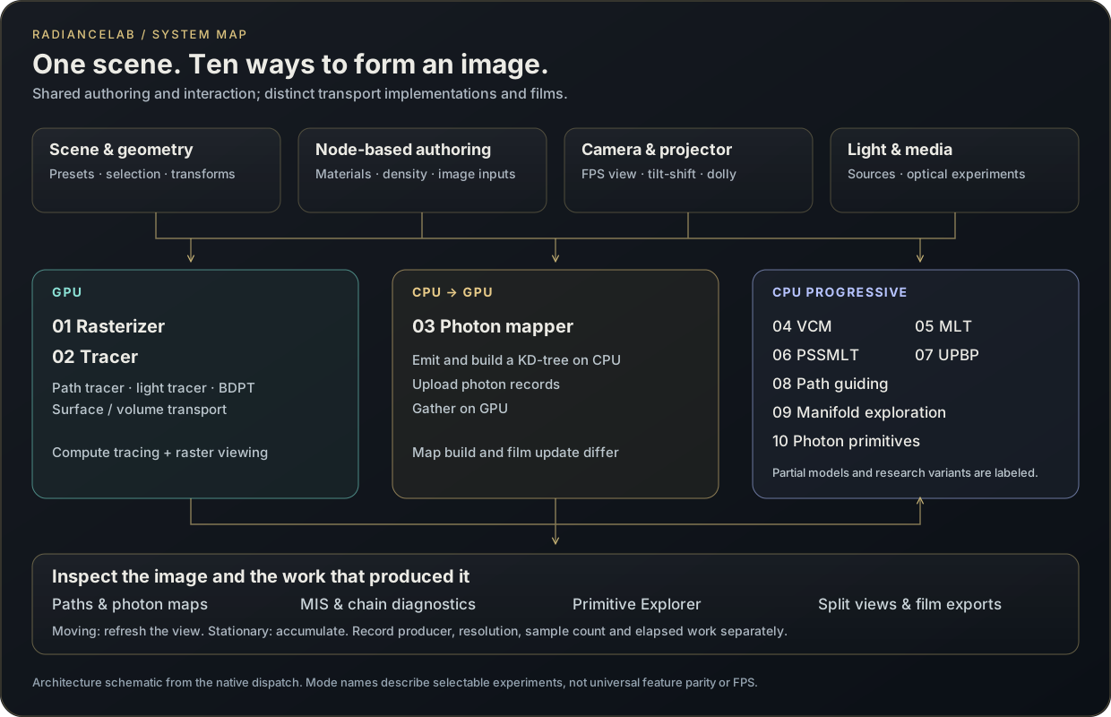
Ten selectable modes share the studio. The GPU tracer contains the path tracer, light tracer and bidirectional path tracer, while the photon-primitive mode contains a separate roster of 34 strategy slots. Rasterization, GPU compute, CPU-built/GPU-gathered photon maps and progressive CPU films provide different routes into the scene; the table identifies what each route currently implements, and the chapters that follow take the methods cluster by cluster.

Architecture schematic derived from the native dispatch. The ten mode numbers match the UI; shared controls do not imply identical material support, film resolution or convergence rate.
Diagram Architecture schematic derived from the native dispatch. The ten mode numbers match the UI; shared controls do not imply identical material support, film resolution or convergence rate.
Mode in the selectorImplementation laneWhat it exposes
01 · RasterizerGPU rasterThe fastest route: plain raster shading draws a complete image every frame; two guided variants composite traced appearance into the raster image.
02 · Path tracer, light tracer and bidirectional path tracerGPU computeSeven light strategies from one compute shader, including live BDPT with a clickable strategy pyramid; the broadest material and medium feature path.
03 · Photon mapperCPU photon build → GPU gatherGlobal and caustic photon maps, KD-tree lookup and progressive radius reduction; cached volume photons for bounded homogeneous media.
04 · VCMCPU progressiveLight–eye vertex connections plus surface photon merging, combined with density-based heuristic weights and a fixed factor.
05 · MLTCPU progressiveBootstrap bright paths, perturb their stored random choices, accept/reject and accumulate splats.
06 · PSSMLTCPU progressiveAn explicit primary-sample-space state, mutation rollback and observable chain statistics.
07 · UPBP (Unifying Points, Beams, and Paths)CPU progressive · subsetSurface connection and merging; in media, collision volumetric path tracing with NEE and a volume-point gather averaged 50/50. Stored beams are drawn but not gathered.
08 · Path guidingCPU progressive · experimentalLearn directional histograms on a spatial grid, then steer later path samples using that field.
09 · Manifold explorationCPU progressive · prototypePrimary-sample Metropolis with smaller perturbations at specular bounces; the Newton constraint solve of published manifold exploration is not built yet.
10 · Photon primitivesCPU progressive · multithreaded34 strategy slots. Hand-picked swept dimensions become a technique with MIS, and stacking gives every transport exactly one owner: the hourglass takes its own paths, a camera walk the rest.
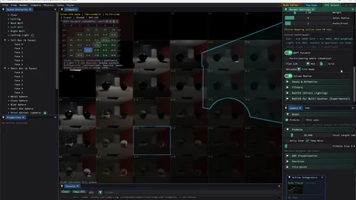
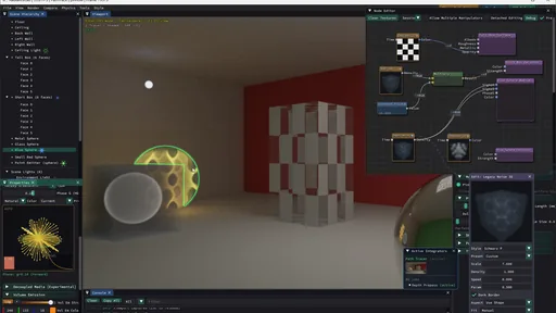
Image Glass, reflective surfaces and a procedural object in the scene editor.
Video One fixed room rendered in turn by the photon mapper, rasterizer, tracer, VCM, MLT, PSSMLT, UPBP, path guiding and manifold exploration, with each mode’s settings and console statistics.
ExplanationComprehensiveness means more than an integrator countMethods, image formation and day-to-day scene work are three complementary design goals.

The breadth pays off in the connections between capabilities: a difficult caustic can be composed visually, investigated through several sample constructions, and rendered with the same scene and camera context.

Ten is the number of top-level selectable modes, not ten independent, complete reproductions of established papers. MLT and PSSMLT currently both use primary-space mutation; UPBP (Unifying Points, Beams, and Paths) and manifold exploration have narrower implementations, described in their chapters. The source therefore supports a broad academic-methods laboratory with explicit experimental branches.

Real-time describes the intended interaction loop. The GPU material preview, a progressive CPU estimator and a converged high-resolution photograph have different costs. Work and resolution controls let those routes remain usable; no universal frame-rate or instantaneous-convergence claim is implied.

Photon primitives are listed as part of the transport dimension but get their own row, because they are a large system in themselves. The photon-primitive chapter (Mode 10) explains how a hand-picked set of swept dimensions becomes a technique, how techniques combine under MIS, and how stacked techniques cover every transport exactly once.

DimensionConcrete scopeWhat it enables
Transport methodsPath tracer, light tracer and bidirectional path tracer; photon mapping and progressive photon mapping; vertex connection and merging (VCM); Unifying Points, Beams, and Paths (UPBP); MLT and PSSMLT; path guiding; manifold exploration; rasterization with traced guidance.Study different routes to the transport integral inside one scene workflow.
Transport methods: photon primitivesAny choice of non-temporal swept dimensions becomes a technique. The roster has 34 strategy slots: every combination of direction angles and flight distance, emitter-coordinate sheets, and refracted, glossy, mesh-sheet and surface-curve constructions.Combine techniques under MIS, and stack them into one hybrid estimator in which every transport has exactly one owner.
Image formation and samplingRGB and spectral tracing; BSDFs and angular/spectral emission; participating media; temporal/spatial reservoir reuse; camera optics; projector and ToF instruments.Express material, lighting and measurement experiments with their actual inputs visible.
Convenient visual workflowFirst-person navigation with a physical camera (tilt-shift, dolly zoom, custom apertures); selection, gizmo and per-object components; typed node editing with previews; live switching among ten modes; a Take a shot photograph; debug views of auxiliary structures and intermediate results.Walk in, change what is visible, switch the estimator under a live preview and take the photograph, with the estimator’s work visible throughout.
Source evidenceTen-mode selection, navigation and camera controlsoffline_projs/RadianceLab/src/core/Engine.cpp
ExplanationA shared scene does not imply an identical estimatorThe rendering modes share an interface but retain their own material support, sampling rules and film outputs.

The difficult integration problem is not placing ten names in a selector. Each backend must agree with the application about scene edits, camera state, film ownership and when accumulated samples become invalid. A camera move must not blend old and new viewpoints. A material change must reach the actual transport implementation, rather than changing only the raster preview. A switch from GPU compute to a progressive CPU film also changes the producer of the displayed image.

RadianceLab makes these producers explicit. The GPU tracer contains the path tracer, light tracer and bidirectional path tracer in one compute shader. Conventional photon mapping builds photon data on the CPU and gathers it on the GPU. The other progressive modes maintain their own CPU films and diagnostic state. Consequently, equal pass counts do not establish equal work: a pass may launch camera paths, build a photon population, run a mutation batch or evaluate many swept primitives.

This separation is useful experimentally. A comparison can first match a supported diffuse or homogeneous-medium scene, then vary the estimator. More elaborate GPU materials and heterogeneous media remain valuable demonstrations, but they cannot serve as a reference for a CPU lane that does not implement the same model. The correct comparison is between matching image-formation contracts, not merely matching scene-file names.

ExplanationFeature specialization is part of the engineering resultPath construction, material support and shader size constrain which combinations can run together.

The GPU tracer specializes around transport features such as bidirectionality, spectral behavior, participating media and explicit path-density MIS. A single maximal shader is not automatically the best implementation: its instruction footprint can exceed the practical limits of the target OpenGL driver. The application therefore starts with a smaller configuration and selects specialized variants as features change.

One consequential boundary is instruction size. If a requested feature mask exceeds the driver budget, the explicit BDPT MIS variant is dropped and the failure is logged, rather than silently rendering a different estimator. Since the BDPT audit, a compact BDPT kernel keeps explicit MIS with one homogeneous medium; other media use a labeled volumetric path-tracing fallback, and finite-aperture camera BDPT still uses flat weights. These are visible feature boundaries, not evidence that surface MIS and medium transport separately fail.

The studio’s system contribution is the inspectable path from control to implementation: which backend runs, which variant was compiled, which film is accumulating, and which diagnostic buffers belong to it. Keeping those distinctions explicit prevents a visually plausible image from silently becoming evidence for a feature that was never enabled.

Source evidenceTransport implementation boundaries ↗Compute-kernel specialization ↗Feature masks and the BDPT MIS variantoffline_projs/RadianceLab/src/render/ComputePathTracer.cpp
Capability family

Photon hourglass: sharp volumetric caustics through glass

An analytic photon primitive draws the light refracted through a glass sphere as a whole sheet, sharp within a second of holding the camera still; traced mesh sheets carry the idea to triangles, with a biased preview for walking.

02 · Photon hourglass · analytical sphere chains

Volumetric caustics through glass, sharp within a second

Description · at a glance

Start with a cone of light. Continue every ray through a glass sphere, following entry and exit refraction, and the outgoing family becomes the hourglass. Its useful trick is to preserve an entire family of paths: the camera intersects a sheet instead of waiting for a nearby photon. The next question is natural: what if the incoming family is a plane?

Light focused by a glass ball and scattered once by fog toward the camera is one of the hardest paths to render: a shadow ray cannot bend through the glass, so a camera path finds this light only by chance, and never under a point light, while a photon beam or point kernel blurs it. The photon hourglass, strategy 20 of the CPU photon-primitive mode, follows both refractions through the sphere exactly and sweeps the exit ray around the axis from the light through the ball’s centre, producing a whole refracted sheet that narrows to a waist and fans out again. A camera ray crosses that sheet by solving a quadratic and collects its contribution at an exact weight, with no kernel radius. Here, photon hourglass means the analytical cone-through-glass construction on spheres and compatible chains. The polygon extension is called mesh sheets; it is kernel-free but uses a numerical surface representation.

It is fast. On the single-ball scene one pass costs 1.2 to 1.5 ms on a 217×140 film on laptop CPU cores, with no GPU compute in the loop. Measured at equal time against photon beams on the same caustic, its variance is 35 to 48 times lower on a two-ball chain and 17 to 21 times lower on a mirror relay. In the recordings the sheet under The Gate’s ball and under a collinear pair is sharp within a second of the camera stopping, at about 150 passes a second on a 524×386 film; restarted in place on the same caustic, photon beams are still grainy after three seconds and photon points barely outline it.

Pairing it with another estimator makes the point sharper. The hourglass owns the caustic, and something else draws the rest: mostly light that reaches the fog directly and scatters once, a far easier path. Yet in the recordings the easy part converges last. After the switch to the hourglass MIS pairing, the lamp’s direct glow is still grainy six seconds later, while the hourglass alone had smoothed the caustic within a second; on The Gate rendered with mesh photon sheets in the next chapter, the directly lit shaft needs two to three seconds after the caustic under the ball is already smooth.

Video The Gate on the analytic hourglass (strategy 20). While the camera walks, the film restarts every frame and the refracted sheet under the glass ball is a scatter of dots; a fraction of a second after it stops the sheet is smooth, with the pass counter climbing by about 150 passes a second on a 524×386 CPU film. Strategy 20 draws only light refracted through the ball, so the shaft through the gate stays dark.
Theory / mathematicsA cone through glass. What about a plane?The central plane can survive intact. Its cheap crossing is only part of the estimator.

For the spherical hourglass, fix the polar angle and sweep azimuth plus outgoing distance. Rotational symmetry turns the refracted family into a surface of revolution with a compact crossing solve. The complementary choice fixes azimuth and sweeps incidence angle plus outgoing distance: a meridian sheet through the light and sphere center. Every ray and surface normal stays in that plane, so both refractions preserve its planarity.

That makes the meridian an interesting candidate, not merely a less elegant hourglass. A camera-plane crossing is cheap, but the crossing point must still belong to the transmitted family. Recovering its incidence angle may require finding several branches near a caustic fold; the sampling density and Jacobian must count all valid paths. A nearly parallel camera ray also makes the plane poorly conditioned. This could complement the hourglass rather than replace it.

A parallel light sheet moved away from the sphere center tells a different story. Its varying normals bend it into a ruled, potentially folded sheet. A flat parallel-sided slab provides a useful control: a parallel ray sheet remains planar after its two refractions. The browser study computes these rays directly and draws their outgoing support and receiver footprint; its luminous shading is a display reconstruction, not a new unbiased transport estimator.

Performance depends on more than how easy the sheet looks to intersect. The existing spherical hourglass can rotate one solved meridian path; a general displaced sheet needs many distinct refraction evaluations and a finite support representation. Conversely, a central meridian offers a very cheap plane cull. Build cost, all-root inversion, visibility and error at equal time determine whether that trade pays. This browser study does not measure an equal-error speedup for the proposed volumetric meridian member.

There is already a related native implementation: surface receiver curves can use cone, meridian plane or a shared-budget mixture of both. That forward surface construction is distinct from the inverse camera-to-volume meridian estimator explored here. The new exhibit makes its geometry visible; it does not substitute for a transport benchmark.

FamilyGeometry that survivesWork that remains
Cone through a sphereRotational sheet / hourglassAdmissible quadric roots, transmitted branch and density
Central meridian through a sphereAn exact planeFinite transmitted support, incidence-angle roots and grazing crossings
Offset parallel sheet through a sphereA curved ruled sheetDistinct refractions, folds, support approximation and weights
Parallel sheet through a flat slabA planeTwo-interface displacement and finite slab support
ExplanationWhy a sheet can resolve a narrow causticEvery camera ray that crosses the sheet collects light, at an exact weight.

A photon beam contributes only to camera rays that pass within its kernel radius, and a photon point only to rays that pass near the point. A refracted sheet is a surface in the fog, so a camera ray collects a contribution wherever it crosses it. In the numerical variance study, 74% of hourglass samples contribute to a fixed camera ray at the waist, against 11% for a beam of radius 0.01. At the waist that thin beam is as good per sample (relative variance 9.3 against 11.3), but below the waist, where the light bundle is wide, its relative variance grows to 92 against 14.5 for the hourglass. Fog density does not change those hit rates.

The equal-time figures come from the linear film, not the displayed image. On the collinear two-ball chain (preset 68), relative variance per pass times milliseconds per pass is 6.8 for the hourglass chain against 241 and 329 for beams of radius 0.12 and 0.06, and the total energy on the caustic agrees with the beam within about 0.6%. On the unfolded mirror leg (preset 71) the equal-time gain is 17.4 and 20.6 times.

Speed has a limit. Two four-ball chains under two lights (preset 77) carry a relative variance of 34 per pass on the caustic: 29% relative error at 400 passes, 15% at 1,600 and 7% at 6,400, which at 50 passes a second is about half a minute and two minutes of holding still. The recording of that scene, in the chains chapter, is still grainy after a few hundred passes, as measured.

Theory / mathematicsAnalytical hourglass and kernel-free mesh sheetsAn exact construction on spheres, a numerical extension to polygons, and a separate fast preview.

The analytical hourglass has an unbiased formulation for the path class it represents: exact refraction, all admissible crossings, the correct Jacobian and sampling density, and no discarded contributions. It estimates that class of transport; another estimator must supply paths outside its support. Mesh sheets extend the construction to polygonal geometry with traced rulings and numerical reconstruction. They avoid a photon-gathering kernel, but kernel-free does not by itself mean unbiased.

The recorded implementation has additional choices. A grazing guard rejects very small Jacobians, off-axis followers search a finite set of rulings, and strategy 21 introduces the finite-radius beam/point kernels of its MIS partners. These choices can introduce bias. The optional screen-raster viewfinder is a further, deliberately biased approximation. These are implementation distinctions, not different names for the same estimator.

Name used hereConstructionScope of the claim
Analytical photon hourglass · strategy 20A cone swept through a sphere or compatible analytical chainUnbiased formulation for its represented path class; guarded or numerically searched implementations need the qualification above.
Mesh photon sheets · strategy 32Traced rulings through polygonal geometry, with numerical sheet reconstructionKernel-free; discretization and numerical crossing errors remain.
Hourglass MIS · strategy 21Analytical hourglass combined with finite-radius kernel estimatorsThe finite-radius mixture carries kernel bias.
Fast structure previewScreen-raster reconstruction of the primitive supportA deliberately biased viewfinder for motion and scene exploration.
Interactive schematic

A cone through glass. A plane through glass.

A cone through glass. A plane through glass.

Compare the hourglass, a central meridian and an offset light sheet. Change the glass and inspect what remains planar.

Draws with Computed Snell geometry · projected with Canvas2D

Artifact Interactive optical geometry study with schematic and luminous views.

Export Prepare image exports the current computed view as PNG.

Purpose Motivate the hourglass and inspect a complementary planar family.

Made with Adapted from RadianceLab’s hourglass coordinate construction; independent browser illustration.

Demonstrates A central meridian stays planar; displaced sheets can bend. Cheap crossing alone does not establish an estimator speedup.

Open separately ↗

Wheel over the scene may zoom; move outside it to scroll the page.

Preview of A cone through glass. A plane through glass.

Computed two-interface Snell geometry and receiver footprints. Luminous shading is a biased display of the sampled sheet; this browser study does not benchmark a complete photon estimator.

Suspended · activate to run; playback pauses after the full panel leaves the vertical viewport.

03 · Eight ideas under exploration · selected successes and revealing failures

Rendering frontier: make the difficult connection easy

Description · at a glance

The hourglass suggests a broader question: what happens when the coordinates themselves follow a difficult connection? A rotational atlas combines cylinders, cones and hyperboloids, with a plane partner for a direction the three can share as a blind spot. A shadow atlas remembers visibility where neighboring primitive queries ask almost the same question.

The two-scatter suite carries a real point-source, phase-function, scattering, attenuation and visibility ledger. The shadow study evaluates an actual occluded sheet field. Alongside them, six smaller browser studies explore medium relays, arrival-time shells, tilted focus, nonlinear reflection constraints, plane–plane intersections and distant path coordinates. These are interesting ideas under exploration: an attractive working case and an instructive failure are enough to reveal their potential.

Selected experiments now run inside RadianceLab’s native research window: the rotational atlas, a bounded three-scatter sheet family and a visibility-cache comparison. Choose a scene, accumulate its film, inspect the subpaths and save the settings with a recording. These controlled renderers remain separate from the general scene integrator; the browser studies explain their related geometric ideas.

Image Rotational Atlas: a restricted exactly-two-scatter film, using three rotational charts and a 10% plane partner. Display reconstruction is optional; the notebook also shows the unfiltered film, individual methods and a separate transport reference.
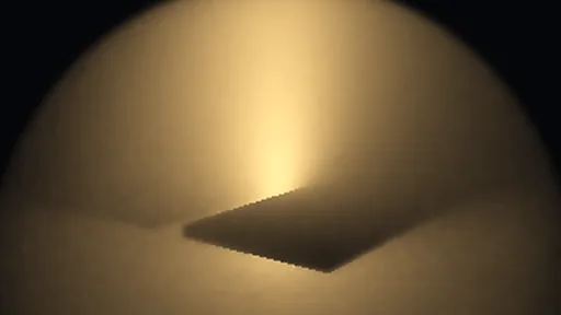
Image Shadow Atlas: actual visibility through a slatted screen projected onto a luminous hyperboloid. False color and bloom show the conditional field; this image is not a full volumetric-radiance render.
Theory / mathematicsEight directions, different levels of implementationWhich ones estimate a physical target, and which ones expose a mechanism?

These names are exhibition titles for experiments within an established family of path-space ideas. The published Photon Surfaces construction supplies the common framework. The numerical notebooks retain linear results separately from display effects, and the browser studies describe their own approximations. No new general-purpose production integrator is implied.

StudyWorking scopeWhat can fail
Rotational AtlasPhysical, bounded, exactly two volume scatters; four-chart MIS.A fixed allocation can lose to one well-matched chart; difficult references may remain noisy.
Shadow AtlasFrozen primitive-coordinate visibility cache with stochastic exact correction.Fine silhouettes and stale geometry increase bias in cache-only mode and variance after correction.
Scattering RelayStructured-medium rendering and endpoint-guided proposal diagnostic.High scattering density alone does not imply useful light–camera transport.
ChronolensPath-length shells and straight-segment optical-distance comparison.Varying index invalidates a purely Euclidean time gate; ray bending is outside the study.
Scheimpflug FanTilted-focus thin-lens rendering study.Large apertures expose occlusion and finite-sampling limitations.
Caustic LoomA small reflection-constraint solve, separate from the active native manifold work.Newton can miss roots or fail; a converged root does not supply a complete transport PDF.
Crossed SheetsFinite plane intersection and conditioning diagnostic.A line still has a dimension to integrate; near-parallel or disjoint supports are problematic.
Path AtlasAdjacent/distant parameter and visibility study.Larger support can create more expensive, occluded or invalid connections.
04 · Photon hourglass · the biased group

Beyond spheres: mesh photon sheets through triangles

The analytic hourglass needs a glass sphere. Mesh photon sheets (strategy 32) drop that requirement by tracing the sheet instead of deriving it. For a sampled light point and azimuth, a fan of rays at finite polar-angle steps is traced through closed triangle meshes and analytic shapes, with refraction, Fresnel weights and total internal reflection. Neighbouring rays with the same history are joined into strips of triangles, and each camera ray gathers the strips it crosses with a projected Jacobian. Suzanne, the Utah teapot, a torus with a hole and chains of different glass bodies all send their own waists and fans into the fog.

What changes is where the error enters. The analytic sheet is exact and only its sampling is noisy; the traced sheet is a finite quadrature of a continuous family of rays, so more passes remove noise but not the discretization. Refining the ruling from 64 to 256 intervals raises the mean image by 15.8% on Suzanne, 13.8% on the torus and 3.7% on three spheres. Topology changes the strips cannot follow, an angle threshold and a grazing cutoff also discard energy, and the mode covers one fog scatter after the glass with a single index of refraction. In exchange, the traced sheets render the off-axis pair that the analytic chain refuses in correlated mode.

A second approximation turns either sheet into a viewfinder. The fast structure preview rasterizes the sheet triangles at reduced resolution with fractional pixel coverage, a small blur and a grazing floor, from a pinhole camera. Folds appear at once and follow the moving camera; the panel labels the result an approximate viewfinder, not a convergence reference.

Video Mesh photon sheets (strategy 32) through closed triangle meshes in fog: Suzanne, the Utah teapot, three triangulated spheres, a torus with a hole and a four-body chain of sphere, oblate and prolate meshes each send their own waists and fans into the fog, followed by walks around the chain, the torus and Suzanne. The sheets are traced rather than derived, so no rotational symmetry is needed; walking frames restart grainy.
05 · Central research example

The hourglass: follow the refracted sheet

Description · at a glance

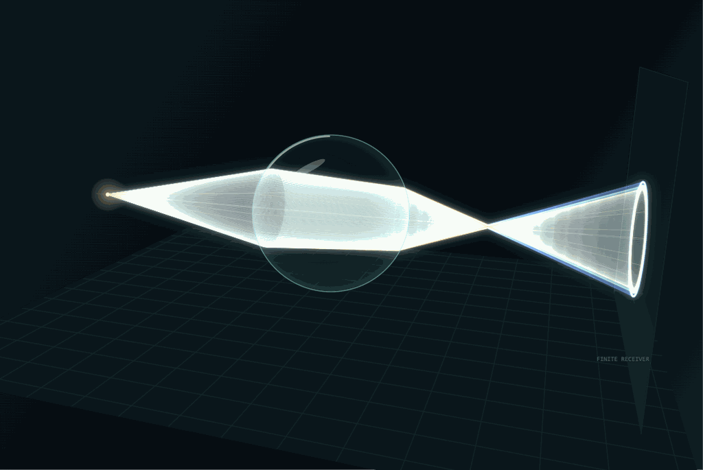
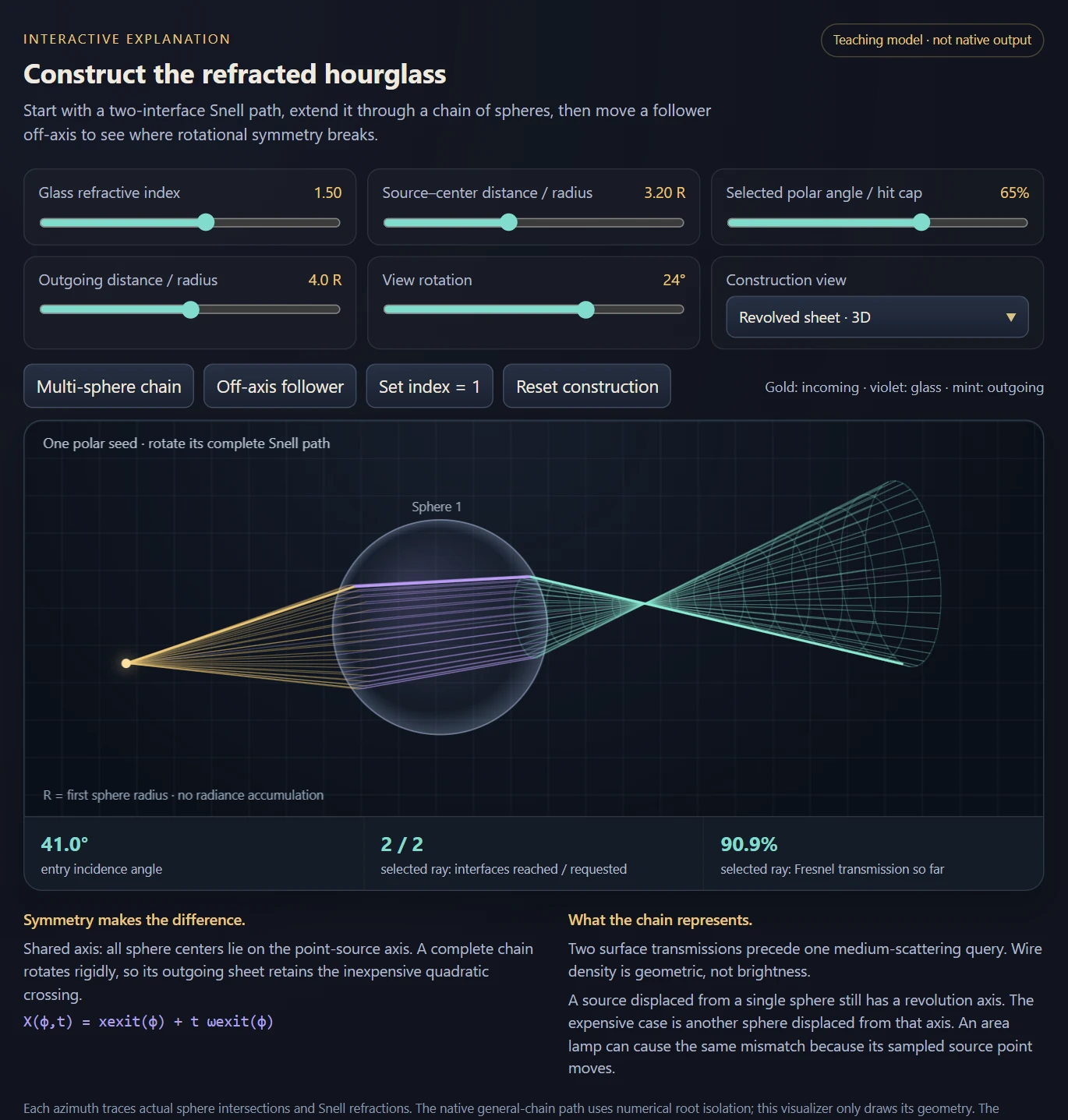
A source and a spherical dielectric define a rotational Snell construction. Sweeping the entry, internal chord and exit together produces a refracted sheet whose camera crossings recover the supported volumetric caustic.

The waist connects geometric focusing to estimator density. The core path has two specular transmissions followed by one medium-scattering event, with an index-one limit that supplies an independent check.

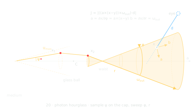
Source-authored construction diagram: sample a polar direction toward the sphere, trace two refractions, and revolve the outgoing ray about the source–sphere axis.
Diagram Source-authored construction diagram: sample a polar direction toward the sphere, trace two refractions, and revolve the outgoing ray about the source–sphere axis.
J=∣[a×(x−y)]×ωout  ⋅d∣J=\left|\left[\mathbf a\times(\mathbf x-\mathbf y)\right]\times\boldsymbol\omega_{\mathrm{out}}\;\cdot\mathbf d\right|
For revolution about axis a through sampled source point y, the two swept tangents are a × (x − y) and the outgoing direction. Their cross product projected onto camera direction d is the co-area factor. The parameterization and branch support are part of this expression.
Image Shared hourglass samples make the refracted ruled surface and its narrow waist directly visible.
Theory / mathematicsThe hourglass sweeps an entire Snell chain by rotational symmetryIts analytic power comes from a precise geometric restriction.

Choose a source point outside a sphere and the axis joining it to the sphere center. A sampled polar direction determines one entry point, one internal chord and one exit direction through two Snell refractions. Rotating that entire path around the source–center axis preserves the sphere and both interfaces. The construction therefore sweeps a family of physically related refracted paths, rather than refracting independent rays and fitting a surface afterward.

After the second interface, sweeping azimuth and outgoing distance forms a ruled sheet. Its narrow waist is a geometric caustic: nearby members of the family approach one another. The camera query solves crossings of this sheet and evaluates the transmission, phase, attenuation and visibility belonging to the crossing’s actual azimuth.

The rotational restriction is essential. A general object or an off-axis follower does not preserve the same family under rotation. Even for a sphere, the implicit quadric contains algebraic branches that are not the forward transmitted ray. The valid nappe, outgoing distance and visibility checks define the estimator’s physical support. Setting the refractive index to one provides a sharp control: the construction should reduce to the corresponding cone family over the same sampled cap.

The hourglass paths are light → transmission at entry → transmission at exit → one volume-scattering event → eye, crossing two interfaces before a single medium event. The hourglass owns these paths and is stacked with other techniques into one estimator for complete transport (see Stacking techniques in the photon-primitive chapter).

X(c,ϕ,r)=xexit(c,ϕ)+r ωexit(c,ϕ)X(c,\phi,r)=x_{\mathrm{exit}}(c,\phi)+r\,\omega_{\mathrm{exit}}(c,\phi)
c=cosψ is the sampled source-side polar coordinate; φ and outgoing distance r are swept. The exit point and direction are obtained from the same two-interface Snell chain.
∂X∂ϕ=a×(X−y),∂X∂r=ωexit\frac{\partial X}{\partial\phi}=a\times(X-y),\qquad \frac{\partial X}{\partial r}=\omega_{\mathrm{exit}}
a is the unit source–sphere axis and y the source. Rotational symmetry gives the azimuth derivative directly; the distance derivative is the outgoing unit ray direction. Their projected cross product supplies the sheet Jacobian.
Theory / mathematicsA cancelled MIS numerator is not the deposited sampling densityDimensional analysis catches an attractive but incorrect shortcut.

To compare the hourglass with a beam or point estimator, it is necessary to ask how the sampled polar coordinate deposits density along the queried camera ray. Sweeping two variables removes their random sampling, but the remaining map from polar coordinate to arclength still contributes a determinant. At a multi-branch crossing, the density sums all compatible branches.

The hourglass sheet Jacobian alone does not supply that arclength PDF. Multiplying it by the polar PDF produces a quantity with the wrong units. That product can appear after a shared three-dimensional determinant cancels between MIS alternatives, but the cancellation is local to a compatible path event and its support. Reusing the simplified numerator as an independent density outside that calculation is invalid.

This distinction also explains why a rough-interface NDF is not a substitute for the smooth hourglass construction. Exact Snell transmission constrains the half-vector at the interface; changing a roughness parameter around that constrained direction does not reproduce the geometric deposited density of the smooth refracted family. The older rough-proxy exploration remains a separate study, not the shipped smooth estimator’s derivation.

D=det⁡ ⁣[∂X∂c,∂X∂ϕ,∂X∂r]D=\det\!\left[\frac{\partial X}{\partial c},\frac{\partial X}{\partial\phi},\frac{\partial X}{\partial r}\right]
D is the full spatial Jacobian of the map from sampled polar coordinate, azimuth and outgoing distance to position. With c and φ dimensionless and r a length, D has units of length squared.
pHG(s∣y,sphere)=∑bpc(cb) Jb∣Db∣p_{\mathrm{HG}}(s\mid y,\mathrm{sphere})=\sum_b p_c(c_b)\,\frac{J_b}{|D_b|}
The sum is over compatible physical branches at ray arclength s. J has length units for the (φ,r) sheet, so J/|D| has inverse-length units as an arclength density should. Sphere-selection and source-selection probabilities are additional factors when sampled.
Interactive schematic

Construct the refracted sheet

Construct the refracted sheet

Vary the source and polar seed, trace a multi-sphere chain, then shift a follower off-axis to reveal the loss of a simple rotational sweep.

Open separately ↗

Wheel over the scene may zoom; move outside it to scroll the page.

Preview of Construct the refracted sheet

Actual sphere intersections and Snell refractions are evaluated for each azimuth. The chain toggles add specular interfaces, not random volume bounces. The three-sphere off-axis setting explores geometry beyond the native two-sphere off-axis solver; the wire sheet does not estimate radiance.

Suspended · activate to run; playback pauses after the full panel leaves the vertical viewport.

Recorded examples · 2Refractive hourglass constructionsA single relay and a chain expose the geometry behind the caustic estimator.
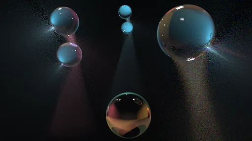
Image An hourglass-estimator scene with several refractive spheres and relay controls. The image exposes the configured construction without claiming a matched reference comparison.
Image Single-sphere hourglass transport with the estimator controls and refracted construction visible.
06 · From derivation to executable geometry

The useful constraint is rotational symmetry

Description · at a glance

Rotational symmetry reduces a camera crossing to a quadratic. The physical branch still needs validation, and near a fold the roots and their Jacobian must remain numerically consistent.

The revised solver shares stable algebra between root classification and weighting. Identical-draw replays, finite differences and limiting tests distinguish floating-point errors from genuine high-variance geometry.

Theory / mathematicsThe solver and the estimator must agree near a double rootThe revised crossing routine stabilizes both the quadratic and the Jacobian derived from it.

Near a caustic fold, two ray–sheet crossings coalesce. The quadratic discriminant becomes small, so subtracting large nearly equal terms can invent a crossing or erase a real one. A separately evaluated Jacobian can suffer a second cancellation and assign an inconsistent weight to the root that survived. A firefly in this region can therefore come from genuine estimator geometry or from an avoidable floating-point inconsistency.

The September solver revision uses a common crossing routine with local double-precision arithmetic, while keeping the surrounding inputs and outputs in the renderer’s usual precision. It normalizes the axis, retains the actual ray-direction norm in the coefficients, shifts the ray parameter near the perpendicular foot relative to the apex, and evaluates a stable paired-root form. The Jacobian is derived from the same factored quantities as the discriminant.

These changes reduce cancellation; they do not introduce exact arithmetic or prove robustness for every possible scene scale. The documented comparison replayed identical draws against the prior solver and recorded root classification and energy changes. Keeping the draws fixed makes that test substantially more informative than comparing two unrelated noisy images.

Δ=B2−4AC,q=−12(B+copysign⁡(Δ,B)),t1=qA,t2=Cq\Delta=B^2-4AC,\quad q=-\frac12\left(B+\operatorname{copysign}(\sqrt\Delta,B)\right),\quad t_1=\frac qA,\quad t_2=\frac Cq
For a nondegenerate quadratic with real roots, the paired form avoids cancellation in one root and obtains the other through their product. Linear cases, repeated roots and q=0 require explicit handling; this expression is not a replacement for those branches.
J2=Δ4wz2J^2=\frac{\Delta}{4w_z^2}
For the documented normalized hourglass sheet coefficients and its nondegenerate axial parameter w_z, the squared crossing Jacobian and discriminant share a factored quantity. The identity explains why evaluating roots and weights through one consistent algebra is valuable; it is specific to this parameterization.
07 · Beyond one sphere

Extend the construction without losing its assumptions

Description · at a glance

Additional interfaces reveal which symmetries keep the construction tractable. Collinear chains retain an analytic route; an off-axis follower requires a more expensive numerical strip search.

Seed, reflection, glossy and camera-leg variants change the represented path class. Their restrictions explain both the working cases and the extensions that need a different construction.

The construction above has independent chain and off-axis controls. A point source and collinear spheres preserve a common axis even through many transmissions. An off-axis follower breaks that symmetry; a sampled area-light point can break it too. The cost increase comes from the crossing problem, not simply the number of glass interfaces.

Image Original embedded plate from the standalone manuscript: preset 79, The Atrium, with three refractive chains and a dispersive sphere. The source labels this a 607 × 447, 400-pass appearance composite; it is not an equal-time reference comparison.
Image Hourglass-estimator scene with multiple refractive spheres and relay controls.
Video An off-axis follower breaks the symmetry. In correlated mode the analytic chain refuses and says why, leaving the film black; with a fresh primitive per sample, a numerical crossing search draws the caustic that reaches the follower, grainy while the camera walks.
Video Two collinear chains of four glass balls under a blue and an amber point light. The analytic hourglass follows the light through every ball, and the sheets narrow to waists between them and fan out below. With eight balls and two lights the film is still grainy after a few hundred passes: this is where the construction’s speed runs out.
ExplanationA longer refractive chain can change the problem classThe boundary between a closed-form sweep and a numerical strip is part of the research result.

A collinear sequence of rotationally symmetric interfaces can preserve the original azimuth sweep: rotate the seed and the complete chain rotates with it. This permits a relatively compact continuation of the hourglass construction. The challenge is then to carry the correct branch, transmission and domain restrictions through every interface.

An off-axis follower sphere breaks that invariance. A rotated ray does not encounter an equivalent cross-section of the next object. The later T3 route therefore traces a numerically varying family and searches ruled-strip crossings under explicit restrictions. Its evaluation cost and failure cases differ from the analytic quadratic. Calling both examples “two spheres” would conceal the key algorithmic distinction.

The chain study consequently records both successful configurations and refusal conditions. Those restrictions are useful information: they identify which transformations preserve a solvable geometric family, which require numerical continuation, and which are outside the current implementation. They also provide concrete future work—broader chain support requires a new parameterization and corresponding density evaluation, not only a more elaborate scene.

Reflection-cone, exit-cone and glossy studies also vary the seed and path class. A glossy vertex adds real directional freedom, so treating it as an ideal mirror changes the problem. Camera-side reflection or refraction introduces additional viewing legs that current chain and correlated configurations do not all support.

ExplanationMoving one follower changes the solver, not just the pictureA rigid rotational chain gives a quadratic. A general ruled chain requires root isolation on the actual refracted map.

On a common point-source axis, tracing one meridian gives the complete azimuth family by rigid rotation. Additional collinear spheres change the seed path and transmission product, while the final outgoing line still sweeps the same quadric class. A source displaced relative to one sphere alone does not destroy this symmetry: its source-to-center line simply becomes the axis.

A follower away from that axis is different. Its entry point, chord, exit point and outgoing direction vary nontrivially with azimuth; some azimuths miss it. The native off-axis solver samples rulings, brackets sign changes of the camera-crossing residual, refines on the true Snell chain, and evaluates a changing Jacobian with finite differences. Grazing root pairs can need an adaptive rescan. Repeated chain evaluation per queried camera ray accounts for much of the extra work.

The native off-axis implementation currently supports one displaced follower, with an uncorrelated query path; it does not have the same reusable correlated/raster bound as the axial chain. The schematic permits a third sphere to make the geometric consequences visible, but does not claim the renderer supports that extra general-chain case. More interfaces in the picture are specular transmissions before a volume query, not a demonstration of arbitrary multiple volume scattering.

F(ϕ)=(xexit(ϕ)−o)⋅(ωexit(ϕ)×d)=0F(\phi)=(x_{\mathrm{exit}}(\phi)-o)\cdot(\omega_{\mathrm{exit}}(\phi)\times d)=0
A general ruled sheet meets the camera ray where the two lines are coplanar. Roots also require forward-distance, branch and visibility checks.
08 · The tridirectional hourglass · for completeness

Change the seed, change which paths are easy

Description · at a glance

The tridirectional hourglass seeds the path on the glass itself: a point on the sphere, then two halves built independently, a light connection traced back to the lamp and a swept exit sheet that the camera meets. Light subpath, sensor subpath and the two-segment chain through the glass are joined at two constraints, which is what the name means; the project uses it for the whole hourglass family, and these are the members that make it literal. The hourglass began in this glass-seeded form, and the light-seeded strategy 20 replaced it: once the camera crossing fixes the azimuth, the light side has no freedom left and must reach the lamp by tracing, which almost never happens with a small lamp and never with a point light, and that first form carried only one of the ball’s two refractions. The vertex members bring the glass seed back with strategy 20’s machinery. Strategy 22 reuses 20’s Snell chain, camera solve and Jacobian with the rotation axis moved to the surface normal through the ball’s centre; the exit cone (23) and the reflection cone (24) are true cones with their apex on the glass, met with the cone solve of strategy 9.

They are less impressive, and the recordings show why. On the same ball and small lamp, strategy 20 draws a solid caustic horn by pass 60 while 22 and 23 still show sparse dots at pass 76. In the rendered lamp-size study, 20 beat 22 at every size tested, by 236 times at a 2.3° lamp down to 1.9 times at a 77° lamp, where the light trace succeeds almost every time and the fold of the sheet sets the remaining gap; the earlier numerical prediction that 22 would overtake 20 on large lamps did not hold in the renderer. The reflection cone (24) is the positive result: to my knowledge, the first analytic sphere-reflection member within the photon-primitive framework, matching the beam’s reflection branch at 0.998 and filling 1.5 times as many pixels, for lamps with an edge of about 1 or more.

The light-size study measures successful closure separately from nonzero weights. It shows why seed choice and light-side importance sampling matter more than adding every variant to one mixture.

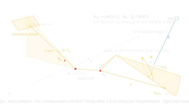
Source-authored entry-seeded construction. At the azimuth selected by the camera crossing, the light-side ray is traced backward; hitting an area emitter is a separate acceptance event.
Diagram Source-authored entry-seeded construction. At the azimuth selected by the camera crossing, the light-side ray is traced backward; hitting an area emitter is a separate acceptance event.

A surface receiver needs another degree of freedom

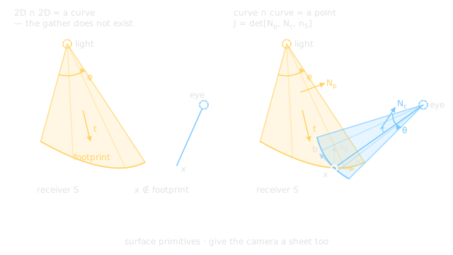
The volumetric construction does not transfer to a wall by merely intersecting the photon sheet with it. That intersection is a curve on the receiver, while a fixed camera hit generally lands elsewhere. The proposed symmetric construction also sweeps a camera sheet, so two footprints can meet on the receiver with a co-area factor involving both sheet normals and the surface normal.

The implemented surface contribution is a simpler reference denominator: a Lambertian next-event connection at the camera’s opaque surface hit, without a continuation bounce in that mode. The two-sheet footprint is a mathematical extension described by the source, not an estimator claimed to be finished.

Image Measured caustic films from the native light-size study: five emitter sizes, each at 2,048 passes. The light-seeded hourglass (20), glass-seeded hourglass (22), full hourglass/beam pairing (21), isolated caustic pairing (21c), and beam reference (18) are shown left to right. Strategy 20 remains better than 22 throughout the tested range; the predicted crossover did not occur. The films use equal pass counts, not equal elapsed time; the printed cost estimates come from short timing runs.
Source-authored proposal, not an implemented result: a photon-sheet footprint generally misses a fixed camera hit; adding a camera sheet changes the incidence problem.
Diagram Source-authored proposal, not an implemented result: a photon-sheet footprint generally misses a fixed camera hit; adding a camera sheet changes the incidence problem.
Theory / mathematicsChanging the seed moves the rare event to a different end of the pathA well-conditioned geometric weight can still lose to a low probability of reaching the emitter.

A light-seeded construction begins with a source sample and asks which refracted family reaches the camera ray. An entry- or exit-seeded construction begins on the sphere and must close the incident direction back to the light. The latter can improve the local geometry of the crossing while making emitter acceptance much worse. These are two distinct components of variance.

A large area light offers a substantial closure region. As the light shrinks, most backward incident rays from a surface seed can miss it. A delta point light is more restrictive still: generic backward directions cannot hit it with nonzero probability. It belongs to a construction that explicitly samples or solves the point-light constraint, rather than one that merely checks a ray against an area emitter.

The source study therefore separates the fraction of samples that close successfully from the distribution of their nonzero weights. This provides a more actionable interpretation than ranking images alone. If acceptance is the bottleneck, improve light-side importance sampling or change the seed. If accepted weights have a severe geometric tail, a complementary construction or a better-conditioned change of variables addresses a different problem.

paccepted(x)=p(x) 1A(x)P(A)p_{\mathrm{accepted}}(x)=\frac{p(x)\,\mathbf1_{\mathcal A}(x)}{P(\mathcal A)}
If a sampler deliberately rejects until it reaches the emitter, its distribution is conditioned on the acceptance set A. The acceptance probability then belongs in the density. Keeping rejected attempts as zero contributions uses a different, unconditioned normalization.
Capability family

Original research: photon-primitive extensions

Extend sampled photons into beams, rings, surfaces and refracted hourglass sheets, carrying their geometry, measure and supported paths through the estimator.

09 · Mode 10 · the research family

Photon primitives: sweep, combine and cover the paths

Description · at a glance

Mode 10 contains the project’s original research: a multithreaded CPU progressive estimator with an optional full-resolution film. A photon primitive samples some coordinates of a light path and sweeps the rest into geometry, such as a beam, ring, sphere, cone, plane or refracted sheet, which the camera ray then queries.

The roster has 34 strategy slots, numbered 0–33. The table shows every way to sweep the direction angles and flight distance of one photon segment, and the emitter-coordinate sheets; further slots add refracted hourglass constructions and their chains, vertex-seeded and glossy variants, MIS mixtures, a rasterized gather, a user-picked pair or trio (31), mesh photon sheets (32) and surface curves (33).

Two ideas turn the roster into a system. Hand-pick the swept dimensions and the framework turns that choice into a technique, weighted under MIS against the techniques that share its measure. Stacking combines them without counting a transport contribution twice: MIS combines compatible overlapping strategies into one estimate, while a hard partition assigns the remaining path classes to a different estimator. The hourglass and a camera walk can then contribute to the same image without both counting the hourglass paths. RadianceLab is the most complete implementation of this photon-primitive framework I am aware of. Earlier reference implementations cover subsets; later work also extends particular parts. The claim concerns the range of primitive constructions brought together here, not universal support for every scene or light path. The construction, measure, variance and validation are developed in the photon-primitive research chapters that follow.

Video Photon-primitive strategies 3 and 7 to 31 on one fog room with a small quad lamp, three glass balls and two reflectors. Each pass draws one shared batch of 16 primitives and each pixel sees one of them, so every type leaves its own geometry: dashed light-quad samples, straight plane fans, beams and points, the refracted caustic horn of the light-seeded hourglass, the same horn as coarse dots for the glass-seeded members, faint reflection-cone fans, a rasterized batch of quads, then rings, arcs and the beam, ring and arc trio.
Swept coordinatesPrimitive (strategy)Support
NothingPhoton point (19)3D kernel
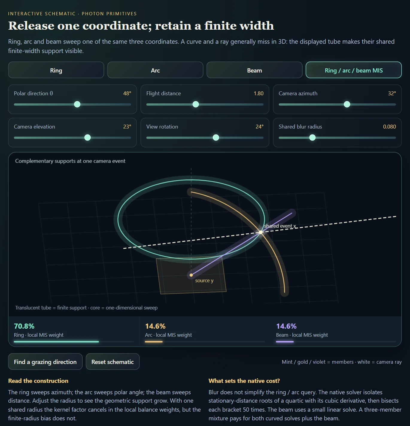
Distance tBeam (18)1D tube kernel
Azimuth φRing (28)1D tube kernel
Polar angle θArc (29)1D tube kernel
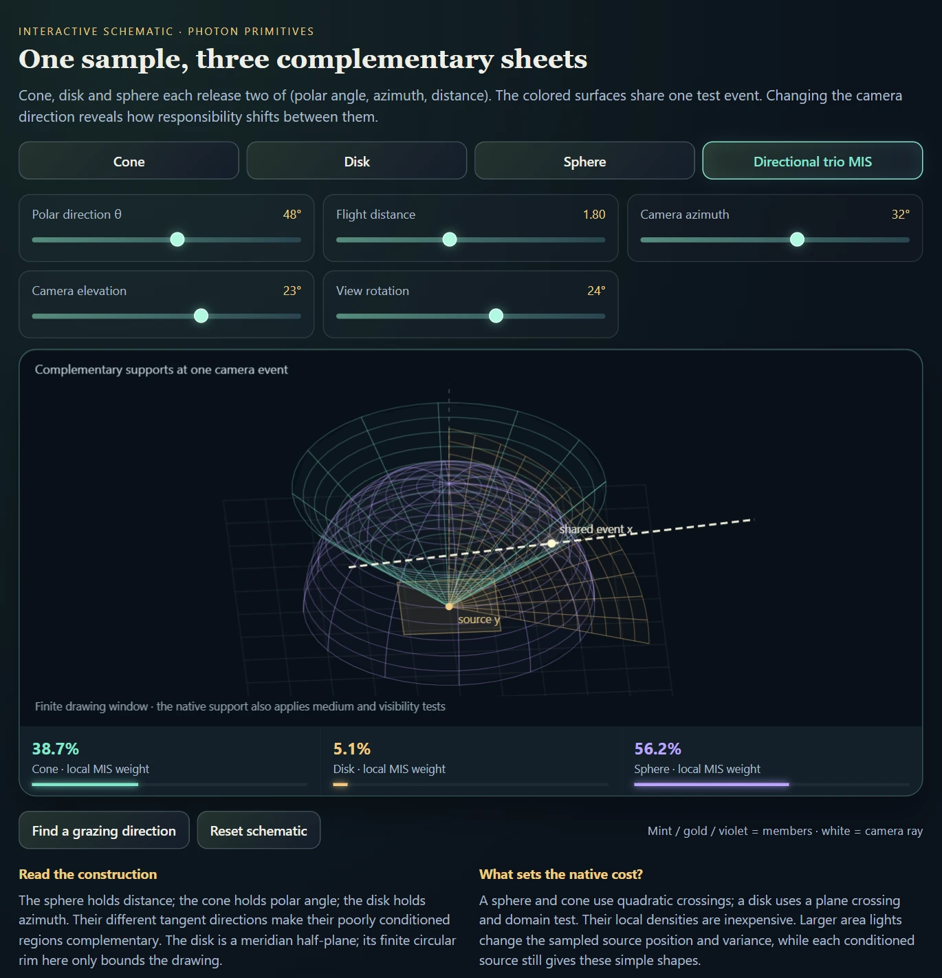
θ and φPhoton sphere (7)Kernel-free sheet
θ and tDisk, a meridian half-plane (8)Kernel-free sheet
φ and tCone (9)Kernel-free sheet
θ, φ and tNEE (1), equivalent to the photon ballExplicit connection: the ball with its distance integrated analytically all the way to the light
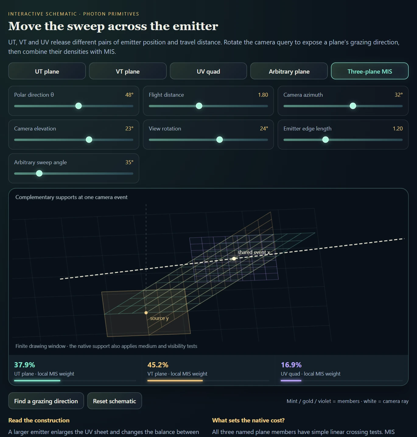
Emitter coordinates, with or without tUV quad and sphere, UVW cube and ball, UT / VT and arbitrary planes (3–6, 10, 11, 14–16)Kernel-free sheets; volume members integrate a chord
ExplanationFrom hand-picked swept dimensions to a technique with MISHand-pick the swept dimensions: the framework classifies the primitive, evaluates it analytically and weights it under MIS, and stacking gives every transport exactly one owner.

Paths sampled from the light and from the camera have to meet, and a single meeting point has zero measure. Connecting the two endpoints fails at specular vertices; blurring them together adds bias. Photon primitives take a third route: sweep, that is integrate analytically, some of the random choices made while building a path. The endpoint then becomes a curve, sheet or volume that the other subpath crosses with nonzero probability. Any choice made during path construction can be swept: the direction angles θ and φ and the flight distance t at any vertex, the emitter’s surface coordinates, or the aperture sample on the camera side.

Once the swept dimensions are picked, the framework builds the technique. A primitive is a list of swept terms, each naming a dimension, the vertex it belongs to and whether it is integrated analytically or sampled. A classifier names the shape: θ and φ at one vertex give a sphere, φ and t a cone, θ and t a disk, all three a ball, two distances a plane, φ at one vertex with t at the next a cylinder, and three distances a parallelepiped. The matching intersector and Jacobian then evaluate it, always through one template: swept dimensions, manifold, crossing roots, Jacobian, contribution. Three free coordinates in total, split between the two subpaths in any way, give an unbiased connection; with fewer, a blur kernel is needed, which is where photon points and beams sit.

Established techniques belong to the same family. The UI names each technique by what it sweeps: L[θφT]=C, with all three coordinates swept on the light side, is NEE (equivalent to the photon ball), and naive path tracing sweeps the light’s own surface and meets the camera ray there. The Photon Primitive Editor draws the idea: toggle θ, φ and distance at any vertex of a camera or light subpath, and it names the shape, shades its Jacobian-weighted density and shows two chosen sweeps combined with the balance heuristic.

Every primitive is a sampling strategy, and techniques combine under MIS by re-evaluation: a primitive pretends to be another one, asks how that technique would have generated the same contributing path, and the balance heuristic weights the densities on a shared measure. Primitives of the same type combine too, such as three planes that sweep different pairs of distances, and so does a continuum of them: arbitrarily oriented planes are MIS-weighted analytically. The best partners behave most differently as the view changes; a photon sphere always has a bright rim, while a plane’s brightness depends on how it faces the camera ray. In the renderer the shared measures group emitter planes on the light-area measure; sphere, disk and cone conditional on the light point; beam, point and hourglass along the camera ray; and beam, ring and arc at one shared radius. Strategy 31 lets you pick your own pair or trio from ten members.

Every non-temporal dimension is supported. Time is the one dimension left out, because a temporal dimension makes the primitive too hard for the algorithm to reason about and adds much more complexity. A time gate removes one more support dimension, so isolated crossings would need three swept coordinates instead of two, and once the camera leg counts, the level set changes from a sphere around the light to an ellipsoid, with an extra coarea factor, degenerate gradients and several branches.

Earlier photon-primitive implementations, including ours from the photon-primitive research project, supported only a handful of these strategies; stock Tungsten, for one, implements photon points, beams and two plane variants.

A technique created this way rarely covers a whole scene on its own, so the next layer stacks techniques into complete transport.

AspectIn RadianceLab
Dimension choiceAny non-temporal swept dimension: directions and distances at any vertex, emitter coordinates and the camera aperture sample; refracted, glossy, mesh-sheet and surface-curve constructions
MISBalance heuristic on shared measures (strategies 12, 13, 15, 21, 26 and 30) and a user-picked pair or trio (31); the camera walk (2) combines phase sampling and NEE with the power heuristic
TimeLeft out
StackingComp mode: a primary technique owns its declared path classes and a camera-walk backup covers the rest; a surface caustic photon map and specular NEE join as further layers, and every transport has exactly one owner
Explanation · 2 media examplesStacking techniques so every transport is covered once and only onceCount each transport contribution once. MIS may combine overlapping sampling strategies; independently summed layers need disjoint path classes.

The rule is about radiance contributions, not the number of sampling strategies. Several strategies may estimate the same path class if MIS combines them with the appropriate weights. What must be avoided is adding two independent, fully weighted estimates of the same transport—for example, a photon beam and a photon plane both counting double scattering. RadianceLab’s Comp mode uses a hard partition between its primary estimator and backup camera walk; the primary may itself contain MIS strategies.

Comp mode renders each pixel with two estimators in the same sample: a primary photon-primitive strategy and a backup camera walk, summed into one radiance, one film and one tone map. Each strategy declares the path classes it owns as a box of counts: non-medium vertices before the first fog scatter (q), fog scatters (nV) and specular vertices between the first scatter and the light (k). The backup multiplies every deposit inside the primary’s box by 0 and every other deposit by 1. Primary and backup estimate disjoint sets of paths, so they add without double counting whatever their correlation, and the declared supported classes have one combined owner. Correct ownership declarations and coverage by the backup remain requirements; the partition alone does not prove complete scene coverage. The hourglass MIS primary (21) weights its beam and point kernel members against the hourglass sheet, so it is consistent rather than unbiased, and the stack keeps its finite-radius bias.

Class counters check the declaration. They print an alarm for any class that receives energy from both layers, the one test that catches a declaration that is too narrow, because a mean image averages that error away. Two more layers follow the same rule: a surface caustic photon map deposits only photons that have passed at least one specular vertex, so surface NEE keeps the direct case, and specular NEE through planar mirrors takes one class over from the walk as a hard hand-over.

Measured with the hourglass MIS strategy (21) as primary and the MIS walk (2) as backup, no class was non-zero on both layers on the test presets, and the primary occupied exactly its declared classes. Seam 0 and seam 1 are two complete partitions and must agree; their ratio was 1.0028 and 1.0060 on presets 48 and 47, against 1.329 and 1.105 with the ownership predicate removed, and 0.9995 on the full hero frame with the specular continuation on. The surface caustic map raised a floor disc’s mean from 0.175 to 21.94 and agreed with an independent first-principles trace to within 2.1%, depending on kernel radius.

LayerPath classes it ownsHow overlap is prevented
Primary: hourglass MIS (21)One fog scatter reached from the light through k specular vertices, k from the seam to the bounce limit minus one (q = 0, nV = 1; k ∈ {1, 2, 3} at seam 1 with four bounces)Declared class box, checked by the class counters
Backup: camera walk (2)Every class outside the primary’s boxDeposits inside the box are multiplied by 0
Surface caustic photon mapSurface caustics after at least one specular vertex (k ≥ 1)Surface NEE keeps k = 0
Specular NEELight → planar mirror → fog scatter → eyeHard hand-over from the walk, not MIS
Video Stacking on film, two off-axis glass pairs under two lamps: for under a second at the start, the console line assigns the refracted caustic to the hourglass (“primary 20 owns …”) and everything else to a backup estimator (“backup 2 fills everything else”). In this showcase setting the directly lit fog is left undrawn under strategy 20, so the dark fog is by design.
Video The Atrium: hourglass caustic plumes stacked over a fully lit room with three lamps and a dispersive hero ball. The backup estimator’s walls and spheres are smooth after a few hundred passes while the plumes are still speckled; each hero caustic receives about a twelfth of the samples.
ExplanationWhat “most complete” refers toCoverage of the photon-primitive family, with a qualified comparison to published implementations.

The comparison is about bringing point, beam, surface and volume constructions, their compatible MIS combinations, and the additional refracted and reflected families into one working environment. It does not imply that every proposed variant is equally robust, or that all scene configurations are supported.

The 2022 reference implementation demonstrates several temporally sliced primitives. DARTS is a later extension of that code for time-of-flight sampling and camera-warped measurements; its supplement explicitly leaves photon balls, volumes and hyper-volumes outside that adaptation. It is a real follow-up, but not evidence of a broader implementation of the whole primitive family.

I have not found a published implementation covering a broader set of this framework. “The most complete implementation I am aware of” preserves that distinction: it is a literature-informed assessment, not a proof that no other implementation exists.

10 · Original photon-primitive research

The representation of a sample changes the problem

Description · at a glance

The central research extension asks how the representation of a sample changes difficult light transport. A narrow caustic may be rarely found by point sampling, while a finite-radius photon estimate spreads energy across the feature. Sweeping selected photon coordinates into geometric support offers another way to reach and resolve those paths.

Photon primitives sample selected variables and sweep the rest into a locus. The camera queries that construction, with density, roots, visibility and supported path classes kept explicit.

Image Recorded hourglass showcase through glass and reflections. This appearance-oriented two-pass composite changes the transport model; controlled estimator films provide the measurement evidence.
Theory / mathematicsPhoton primitives replace selected random choices with a geometric queryThe organizing question is which variables are sampled and which remain integrated.

A scattering step in a homogeneous three-dimensional medium can be parameterized by two outgoing direction coordinates and a free-flight distance. A conventional walk samples all three. A photon primitive samples some variables and lets others range continuously, producing a geometric locus of possible positions. The camera ray then queries that locus.

This is a change in how the same transport integral is represented. A sphere can sweep both direction coordinates at a fixed distance; a cone can sweep azimuth and distance at a fixed polar angle; a plane can arise from an emitter coordinate and distance. The geometric construction pays for fewer random choices with a crossing problem, a Jacobian and a support test.

The word analytic must be read at that boundary. A closed-form crossing does not analytically solve every material, visibility event or radiometric factor. It evaluates a constrained family efficiently and leaves the remaining sampled variables and transport terms explicit. The construction becomes valuable when its integrated variables are exactly those that a random walk would otherwise struggle to coordinate.

X(ξ):Rk→R3,R(s)=o+s dX(\boldsymbol\xi):\mathbb R^k\to\mathbb R^3,\qquad R(s)=o+s\,d
The swept parameters ξ form a k-dimensional locus X. R is a camera ray, with origin o, unit direction d and arclength s. Random unswept parameters are held fixed for this query.
dim⁡(X∩R)=k+1−3=k−2\dim(X\cap R)=k+1-3=k-2
For generic transverse configurations, a two-dimensional sheet meets a ray at isolated roots, while a three-dimensional region meets it along intervals. Lower-dimensional loci require a kernel or another specialized measure; tangencies are exceptional cases.
Swept dimensionRepresentative locusCamera-ray consequence
0PointExact coincidence is nongeneric; a density kernel supplies support.
1Beam, ring or arcA transverse neighborhood enables a curve query.
2Sphere, cone, disk, emitter sheet or hourglassSolve isolated crossings and include the crossing Jacobian.
3Solid region, such as the photon ball (equivalent to NEE)The intersection retains a one-dimensional integral along the ray.
11 · Mathematical model

Geometry only becomes an estimator after weighting

Description · at a glance

A swept primitive is a change of measure. Its contribution depends on how its parameterized geometry crosses a viewing ray, together with the source, scattering, attenuation and variables still sampled.

The dimensional framework builds on Photon Surfaces (2019) and its follow-ups: any hand-picked set of swept dimensions becomes an estimator once its crossings carry the right Jacobian. The refracted hourglass is the project’s own extension, and the derivations and tests identify its specific assumptions.

L^=1N∑i=1N∑r∈RiFi,rpi ∣Ji,r∣\widehat L=\frac{1}{N}\sum_{i=1}^{N}\sum_{r\in\mathcal R_i}\frac{F_{i,r}}{p_i\,|J_{i,r}|}
Schematic crossing estimator: N counts all draws, R contains the valid roots of each draw, p is the remaining sampling density, and J is the co-area Jacobian. F includes the appropriate transport and visibility factors. Individual families have different parameterizations and support conditions.
Theory / mathematicsGeneralized connections turn sampled constraints into geometric crossingsA geometric hit is only the beginning of a valid contribution.

For a two-parameter sheet, the two surface derivatives span an infinitesimal parallelogram. Projecting its oriented area onto the camera direction gives the rate at which sheet parameter area crosses ray arclength. Its absolute value is the geometric denominator of the change of variables. Small values correspond to a grazing or nearly folded crossing.

Every admissible root contributes. A quadratic or quartic can contain several valid crossings as well as algebraic roots outside the primitive’s physical branch. Roots behind the camera, outside the swept interval, on a mirrored cone nappe or occluded along the constructed path must be classified by the same support definition used in the estimator’s density.

The parameterization also determines which probability factors belong in the weight. A sweep uniform in polar angle is not uniform in solid angle. A sweep uniform in cosθ already absorbs the spherical sine factor. Warping a uniform random coordinate into an angle and then multiplying both the warp Jacobian and the same angle PDF counts the conversion twice. The unified notes treat those conversions as explicit entries in a density ledger.

The camera side also determines which variables remain available. A point connection begins at an already sampled medium vertex; a ray connection keeps the camera-distance coordinate free and queries a primitive along that segment. The latter can integrate an event that the former must discover through a sampled distance. Its camera throughput must therefore be taken before consuming that distance law, with the corresponding survival and scattering terms included exactly once. This is the generalized-connection viewpoint: the geometric query and the remaining random choices must be derived together.

J(α,β)=∣(∂X∂α×∂X∂β)⋅d∣J(\alpha,\beta)=\left|\left(\frac{\partial X}{\partial\alpha}\times\frac{\partial X}{\partial\beta}\right)\cdot d\right|
J is the projected sheet Jacobian for parameters α and β and unit camera direction d. Its units depend on those parameters; that dependence must agree with the remaining density factors.
L^η(R)=1pη(η)∑b∈B(η,R)F(η,αb,βb)Jb\widehat L_{\eta}(R)=\frac{1}{p_{\eta}(\eta)}\sum_{b\in\mathcal B(\eta,R)}\frac{F(\eta,\alpha_b,\beta_b)}{J_b}
η collects unswept sampled variables. F denotes the complete radiometric integrand under the specified parameter measure, and B contains all physically admissible roots. This schematic formula requires the sampling and sweep conventions to be stated together.
dω=sin⁡θ dθ dϕ=∣d(cos⁡θ)∣ dϕ\mathrm d\omega=\sin\theta\,\mathrm d\theta\,\mathrm d\phi=|\mathrm d(\cos\theta)|\,\mathrm d\phi
A polar-angle parameter and a cosine-polar parameter carry different differential factors. Choosing either is valid; mixing their weights is not.
12 · Algorithm map

Read the family by what is swept

Description · at a glance

The strategy table has 34 slots, numbered 0–33, including walk baselines, mixed strategies, a rasterized gather route and a user-picked combination. The taxonomy that matters is the geometric support and the paths each estimator represents.

Straight connection families expose how emitter coordinates, directions, and distance can be exchanged for geometry. Refracted constructions add the constraints of a specular chain. Beams, points, rings, and arcs make finite-width support explicit. These distinctions explain both the visual character of low-sample images and the different limiting behavior as work or kernel radius changes.

Source-authored schematic: complementary two-coordinate sheets above one-coordinate ring, arc and beam constructions. The blue ray is the camera query; warm geometry is swept photon support.
Diagram Source-authored schematic: complementary two-coordinate sheets above one-coordinate ring, arc and beam constructions. The blue ray is the camera query; warm geometry is swept photon support.

A dimensional lattice, rather than a list of shapes

At a photon vertex, consider two direction coordinates and one flight distance. Holding distance and sweeping both angles gives a sphere. Holding polar angle and sweeping azimuth and distance gives a cone. Holding azimuth and sweeping polar angle and distance gives a meridian half-plane, called the disk member in the implementation. These are the three complementary ways to sweep two of the three coordinates.

A camera ray and a two-dimensional sheet in three-dimensional space generically meet at isolated points. A curve and a ray generally miss each other, so the one-coordinate ring, arc and beam constructions need finite-width support. The familiar beam is consequently one column of a larger construction. The same count holds for sweeps at any vertex, on the emitter or at the camera aperture; the photon-primitive chapter (Mode 10) gives the general rule.

One-coordinate members have a different solver and a different cost

The ring sweeps azimuth at fixed polar angle and distance; the arc sweeps polar angle at fixed azimuth and distance. Their finite-width circle geometry leads to a stationary-point equation that squares to a quartic. The implementation brackets the roots using the cubic derivative and bisects monotone intervals. All relevant stationary branches must be retained; a nearest-point-only shortcut changes the estimate.

The measured fixed ring/arc/beam mixture suppresses the individual sweeps’ strongest bright outliers, but it draws three light paths per pass. On the recorded unobstructed single-scatter rig it loses to the plain beam on equal time. The documented harder occlusion/emission cases remain future measurements, so robustness in that test is the established benefit.

Why a larger light need not make planes win

There are two different questions: how expensive is one pass, and how many passes are needed for a clean image? The directional trio retains simple sphere, cone and plane queries. The ring and arc solve a more expensive stationary-distance problem even when their width makes the result look smooth. Blur changes support and bias; it does not turn the curved query into a beam query.

A larger emitter helps the planes by expanding their geometric support. The directional mixture is already robust against the members’ complementary tangencies, however, so moving the sampled source across a large emitter need not increase its variance very much. The project’s light-size series exhibits precisely this outcome: the predicted plane/directional crossover was not reached within the tested range. It is a scene-dependent result, not a ranking implied by the shapes alone.

GroupExamplesWhat to inspect
Walk baselinesCamera, NEE, MIS walksCoverage of paths without a specially chosen swept manifold.
Emitter-coordinate constructionsUV quad, UT / VT planesHow emitter position and distance become a geometric crossing.
Direction constructionsSphere, disk, cone, direction mixturesTangency patterns and complementary singular regions.
Specular constructionsHourglass, vertex / exit / reflection variantsRefractive constraints, root branches and the caustic waist.
Finite-radius constructionsTracer beams, points, rings and arcsKernel width, bias and the sample budget needed as width shrinks.
Shared-work routeCached records / rasterized gatherWhether reuse preserves the selected estimator and its normalization.
Selection and receiversCustom pair or trio (31), mesh photon sheets (32), surface curves (33)Which members are combined, and which receiver or sheet construction supplies the support.
Image A correlated photon-sphere visualization: the geometric support remains visible before averaging.
Image A plane-family visualization from the same diagnostic collection. Primitive structure is distinct from a converged radiance film.
Image Photon-ring structure with fixed blur width and a 16-primitive stippled batch.
Image Photon-arc structure with correlated-batch and blur-width controls.
Theory / mathematicsRings and arcs integrate a different variable from a beamTheir shared curve-kernel structure makes the remaining normalization visible.

A beam sweeps distance along one direction. A ring instead fixes polar angle and distance and sweeps azimuth; an arc fixes azimuth and distance and sweeps polar angle. They are different one-dimensional integrations of a scattering step, not three decorative ways to draw the same sample. Their radius and axis show exactly which coordinate has been integrated.

A camera ray and a one-dimensional curve do not generically intersect in three dimensions. The documented estimators use a finite transverse support and a curve–ray Jacobian. The derivative of a unit-speed beam differs from the derivative of a ring parameterized by angle: the latter includes its physical radius. Removing that factor would make brightness depend incorrectly on the curve’s scale.

The ring / arc query also exposes a useful numerical pattern. Squaring the stationary-distance condition produces a quartic, but loses a sign condition. The solver isolates candidates on a bounded interval, refines roots and restores the original condition. All admissible stationary branches specified by the estimator must be considered. The broad-scattering ring/arc modes are distinct from the reflection-cone ring variant, whose specular construction and support are different.

Xring(ϕ)=y+tcos⁡θ a+tsin⁡θ(cos⁡ϕ e1+sin⁡ϕ e2)X_{\mathrm{ring}}(\phi)=y+t\cos\theta\,a+t\sin\theta(\cos\phi\,e_1+\sin\phi\,e_2)
y is the seed, a its axis, and e₁,e₂ an orthonormal transverse basis. With t and θ fixed, azimuth φ traces a circle of radius t sinθ.
Jcurve=∣dXdu×d∣J_{\mathrm{curve}}=\left|\frac{\mathrm dX}{\mathrm du}\times d\right|
u is the curve parameter and d the unit camera direction. The derivative carries the parameter-to-length conversion. The finite-width kernel supplies the additional transverse normalization; the Jacobian alone is not a complete estimator.
Theory / mathematicsA signed-area bug can masquerade as a sampling biasThe arbitrary-plane study separates geometric orientation from probability normalization.

Emitter-coordinate planes are useful because a light coordinate and a travel distance can form a simple swept sheet. Generalizing an axis-aligned construction to an arbitrary orientation creates two separate obligations: preserve the geometric map and derive the density under the chosen emitter coordinates. A result that is too bright or too dark does not identify which obligation failed.

The project’s arbitrary-orientation note records a resolved example. The failure came from using an unsigned area in oriented barycentric coordinates. Reversing the emitter winding changed the numerator signs while the denominator stayed positive, rejecting valid light-domain samples. Tests with a conveniently oriented unit square did not expose that asymmetry.

The correction retains the signed area for coordinate reconstruction and uses absolute values only where a nonnegative density or geometric magnitude is required. This is an instructive robustness test for any generalized connection: rotate the scene, reverse an equivalent parameterization and verify that physical radiance remains unchanged. A successful normalization derivation cannot rescue an incorrect domain-membership test.

As=(eu×ev)⋅nLA_s=(e_u\times e_v)\cdot n_L
e_u and e_v are the emitter’s coordinate edges and n_L the orientation used by the plane construction. Coordinate ratios must retain the consistent signed denominator A_s; replacing it indiscriminately by |e_u×e_v| changes the map under reversed winding.
ExplanationMeasured convergence, solver cost, and the large-light resultSeparate the cost of a crossing from the number of crossings needed; the recorded rig supports the observation without making it universal.

The ring and arc share a stationary-distance solver. Its squared equation is quartic; the real roots of the cubic derivative split a guaranteed bracket into monotone intervals. Each sign change is refined with 50 bisections, followed by restoration of the sign condition lost during squaring. More than one admissible stationary point can contribute. The beam’s small linear solve and the directional trio’s quadratic/planar queries do much less work per candidate.

On the recorded unobstructed single-scatter rig at radius 0.15, the ring/arc/beam mixture reduced median relative variance per pass from the beam’s 108.0 to 39.0. Its mean pass cost was 7.447 ± 0.357 ms versus 1.073 ± 0.062 ms for the beam. Multiplying variance by pass cost gives 290 ± 14 versus 116 ± 7: a smoother pass still lost on equal time. The quoted timing uncertainty is the recorded run-to-run spread; the combined uncertainty does not include an error bar on median variance. These are historical measurements of one native rig, not browser benchmarks.

The constant-power light-size series used a 217 × 140 film and emitter edge lengths from 0.2 to 8.0. Median relative variance per pass for three-plane MIS fell from 135.67 to 3.22. The directional trio rose only from 1.10 to 1.49. Expanding the light helped the planes strongly, but the directional mixture’s complementary densities suppressed the moving singularities better than the initial prediction expected.

At the largest light the reported equal-time products were 4.7 ± 1.4 for planes and 3.6 ± 0.35 for the directional trio. That separation is too small relative to timing uncertainty to claim a decisive speed advantage. The six-member cross-family mixture had the lowest measured per-pass variance, 0.92, but also paid for more queries. In this easy directly connectable single-scatter setup, conventional NEE was a stronger baseline than either family. Visibility, phase anisotropy, kernel width, source size and the chosen error statistic can all change the ordering.

ConstructionNative crossing workWhat MIS changes
UT / VT / UVLinear sheet crossing + emitter-domain checksReduces sensitivity to any one grazing orientation
Cone / disk / sphereQuadratic / planar roots + support checksCombines complementary local densities without a kernel
Ring / arc / beamTwo curved stationary-root solves + beam solveReduces outliers; retains finite-radius bias and extra solver cost
Interactive schematic

Emitter-coordinate planes: UT, VT, UV and orientation

Emitter-coordinate planes: UT, VT, UV and orientation

Change emitter size and camera direction; compare the three coordinate planes, an arbitrary orientation, and their local balance weights.

Open separately ↗

Wheel over the scene may zoom; move outside it to scroll the page.

Preview of Emitter-coordinate planes: UT, VT, UV and orientation

Computed 3D support and native shared-event density numerators. The arbitrary plane is a separate orientation probe; the MIS option combines UT, VT and UV. No native film or timing runs in this schematic.

Suspended · activate to run; playback pauses after the full panel leaves the vertical viewport.

Interactive schematic

Directional sheets: cone, disk, sphere and trio MIS

Directional sheets: cone, disk, sphere and trio MIS

Inspect three complementary two-coordinate sweeps at the same event. A grazing camera direction shifts responsibility to the other members.

Open separately ↗

Wheel over the scene may zoom; move outside it to scroll the page.

Preview of Directional sheets: cone, disk, sphere and trio MIS

The displayed MIS percentages are computed local camera-arclength density ratios conditional on a source point. Wire brightness is schematic; it is not an estimate of image intensity or convergence.

Suspended · activate to run; playback pauses after the full panel leaves the vertical viewport.

Interactive schematic

One-dimensional supports: ring, arc, beam and trio MIS

One-dimensional supports: ring, arc, beam and trio MIS

Compare the released coordinate, change the shared tube radius, and inspect the complementary curve tangents and limiting MIS weights.

Open separately ↗

Wheel over the scene may zoom; move outside it to scroll the page.

Preview of One-dimensional supports: ring, arc, beam and trio MIS

Finite-width tubes illustrate support. The computed weights use the common-event limit; the native finite-radius mixture retains smoothing bias and is consistent as radius shrinks.

Suspended · activate to run; playback pauses after the full panel leaves the vertical viewport.

Recorded examples · 7Photon primitive familiesSphere, disk and cone views expose the support and accumulation of different constructions.
Image The fast-medium experiment with its photon-primitive estimator controls visible. The image records one configured result; the title-bar FPS is not a controlled performance comparison.
Image An early photon-disk film retains the visible sample structure during accumulation.
Image An early photon-sphere film exposes sparse sample contributions before further accumulation.
Image Photon-cone controls with the comparison tooltip explaining the selected inspection option.
Image Photon-cone accumulation with the film and estimator configuration shown together.
Image Photon-sphere accumulation with its film controls and sampled contribution shapes.
Image Photon-disk accumulation with the film controls and primitive support visible.
13 · Reuse and visualization

Correlated sampling as an inspection tool

Description · at a glance

Correlated evaluation lets many pixels query one primitive pool, making sheets, arcs and footprints visible in low-sample images. Freezing and resampling the pool separates the construction from a particular draw.

Correct reuse keeps the total-draw normalization and changes spatial covariance. Cached records and conservative gathering investigate when shared construction also reduces execution cost.

Image The recorded frozen direction-trio pool under equal weights. Individual sphere/cone boundaries remain bright.
Image The same recorded pool under balance weights. Geometry and seeds stay fixed while the weighting suppresses singular rims.
Theory / mathematicsA shared photon population changes covariance, not the marginal targetThe denominator is the number of draws, including the ones that miss.

In independent sampling, each pixel generates its own primitive population. In correlated sampling, many pixels query the same population. For any fixed pixel, the Monte Carlo sum still estimates the same expectation if the primitive distribution, crossing function and normalization are unchanged. What changes is the relationship between pixels: a single sampled primitive can create a coherent feature across the image.

The normalization is the total number of primitive draws, including samples that miss the pixel or fail to form a contributing primitive. Dividing by the number of crossings conditions on success and biases the estimate. Similarly, drawing until a fixed number of valid primitives is reached requires the acceptance probability to be accounted for. A valid record count and a sample count are different quantities.

Keeping one pool frozen across many camera passes is useful for investigating spatial patterns, but it converges to the conditional result of that finite pool. Fresh light pools are needed to average over light-side uncertainty. Camera jitter and light-pool random streams should also remain distinct, so changing image-space sampling does not accidentally redefine the shared light experiment.

L^p=1N∑i=1NF(πi;rp)\widehat L_p=\frac1N\sum_{i=1}^{N}F(\pi_i;r_p)
π_i is one primitive drawn from the chosen light-side distribution; r_p is the pixel’s ray. F includes all valid crossings and is zero on a miss. The denominator N counts draws, not hits or retained records.
Cov⁡(L^p,L^q)=1NCov⁡(Fp,Fq)\operatorname{Cov}(\widehat L_p,\widehat L_q)=\frac1N\operatorname{Cov}(F_p,F_q)
For independent primitive draws shared between pixels p and q, covariance decreases as 1/N when the second moments exist. This does not imply independent-looking noise, and heavy-tailed constructions require additional care.
Theory / mathematicsReuse is valuable when it amortizes construction without changing supportThe speed question and the statistical question have separate answers.

A shared pool can avoid rebuilding an expensive primitive for every pixel. Rasterization or a spatial bound can then restrict evaluation to rays that might cross it. This is a reordering of the same sum only if the footprint is conservative, every relevant root is retained, and the same ray, primitive weight and total-draw normalization are used.

Curved sheets make that condition nontrivial. A polygonal footprint is not automatically a conservative bound on a curved caustic. Missing even a narrow part of the support can remove energy systematically while making the renderer faster. The cached-record and rasterized routes therefore have explicit supported subsets rather than claiming one acceleration structure works unchanged for every primitive.

At a fixed total primitive-evaluation budget, a larger light pool also means fewer camera-jitter realizations if each pass uses one camera sample. That can worsen edges, depth of field or other camera-side variation even while improving the conditional light estimate. The best pool size depends on which source of variation dominates, as well as construction cost and footprint size.

Var⁡(L^)≈NBVar⁡r ⁣(Eπ[F∣r])+1BEr ⁣[Var⁡π(F∣r)]\operatorname{Var}(\widehat L)\approx\frac{N}{B}\operatorname{Var}_r\!\left(\mathbb E_\pi[F\mid r]\right)+\frac1B\mathbb E_r\!\left[\operatorname{Var}_\pi(F\mid r)\right]
For B total primitive evaluations arranged into independent passes of N primitives and one camera ray per pass, the law of total variance separates camera-side and light-side uncertainty. The first term grows with N at fixed B. This model assumes finite moments and the stated independent-pass sampling.
Tshared≈N(cbuild+cbound)+N φ P cqueryT_{\mathrm{shared}}\approx N(c_{\mathrm{build}}+c_{\mathrm{bound}})+N\,\varphi\,P\,c_{\mathrm{query}}
P is the number of pixel rays and φ the fraction covered by a conservative footprint. Reuse can amortize construction, but a large footprint or expensive query can still dominate. This is a cost model, not a measured universal speedup.
Recorded examples · 8Correlated samples and frozen geometryRead the individual primitive shapes before averaging them into a film.
Image Rasterized UV-light quads reveal the structure of a correlated primitive batch.
Image Photon-ring structure with fixed blur width and a 16-primitive stippled batch.
Image Photon-arc structure with correlated-batch and blur-width controls.
Image An arbitrary-plane primitive batch reveals the spatial structure of correlated sampling.
Image Photon-sphere transport with the scene outline retained to locate the inspected objects.
Image A frozen photon-cone batch preserves the same sample geometry while its appearance is inspected.
Image The photon-disk batch-size control links the number of shared primitives to the visible image structure.
Image The photon-sphere batch-size control exposes the shared-sample construction.
14 · Unpublished follow-ups · native receiver experiments

Make the support produce an image

Description · at a glance

A residual circle, a moving boundary and an interference field are more useful when they predict an image on real geometry. These deliberately small native experiments keep the construction inspectable: use the geometry schematic for intuition, then compare its scene result and numerical reference.

Sphere × sphere now samples a genuine scattering connection and compares its film with an independent camera-ray reference. The sharp-boundary experiment moves a collimated quad above a floor and spheres: red enters the light footprint; blue leaves it. The coherent receiver experiment evaluates actual complex fields on curved surfaces: changing relative phase moves the fringes while an incoherent comparison stays unchanged.

Open the native Optics & primitive laboratory from View, or use Sphere-Connection.bat, Sharp-Boundary-Derivative.bat and Coherent-Receivers.bat. These additive fixtures preserve the earlier laboratories and current scene. They are real native computations with deliberately bounded scope, not browser-hosted versions of the renderer.

Image Native sphere-connection radiance: two normalized radial gates isolate a residual circle family in a bounded scattering medium. Both leg visibilities and attenuation are evaluated. 480 × 300, 24 million attempted pairs; no decorative curve drawing.
Image Native scalar-wave receiver render: two spherical fields interfere on a floor and two curved probes. No stripe texture. The warm palette displays relative intensity; the probes do not re-scatter or occlude the optical field.
Image Native sharp boundary derivative over dim original illumination. Red = positive change; blue = negative. There is no chosen world-space blur width: the zero-width boundary measure is integrated over the finite film pixel.
Video Surface curves (strategy 33): photon sheets intersected with the real scene surfaces. The plane meridian sweep draws radial streaks across the ground and the cone azimuth sweep draws loops around the spheres, each with stochastic path samples and with the biased finite curve quadrature; with “Caustic paths only”, just the dotted caustic under the glass sphere remains.
Theory / mathematicsUse the residual circle as a sampling domainThe camera model and both transport legs remain part of the estimator.

Sample a source distance and a sensor distance, intersect the two spheres, then sample an azimuth on the remaining circle. The scattering point carries source intensity, normalized phase function, both transmittances and both visibility tests. Sensor projection and pixel solid angle convert its contribution to the declared radiance film.

For these regular spheres, circle circumference and the crossing Jacobian share a vanishing factor. Their ratio has a stable algebraic form. That is a specific justified cancellation; it does not license dividing arbitrary infinities. Disjoint, nested, occluded and off-screen draws remain in the normalization.

The independent reference integrates along camera rays without constructing circles or evaluating this Jacobian. The published fixtures compare bounded fog, a forward-scattering beam and normalized radial gates. This confirms a restricted working connection estimator, not universal efficiency or support for arbitrary loaded scenes.

J=∣nl×nc∣=ρdrlrc,2πρJ=2πrlrcdJ=|n_l\times n_c|=\frac{\rho d}{r_l r_c},\qquad\frac{2\pi\rho}{J}=\frac{2\pi r_l r_c}{d}
ρ is intersection-circle radius; d is the source–sensor separation. The implementation evaluates the simplified ratio on regular intersections and rejects nonregular cases.
Explanation · 1 media examplesWhere did the width come from?Separate the source kernel, finite displacement and finite sensor pixel.

The older footprint laboratory deliberately smoothed emitter edges; its “thin sheet” retained a finite band. A central difference also produces a finite displacement band even when the source is sharp. PP33’s optional screen Gaussian is a third, separate choice. None of those is required by the mathematical sharp boundary.

The new derivative integrates the sharp boundary through a pixel footprint. Translation along one edge direction activates two opposite quad edges; a general in-plane vector can activate all four. Their extruded planes meet the receiver in curves. A finite pixel receives a finite contribution even though the geometric curve has no width.

The source remains collimated, with fixed receiver response and transport. Curved surfaces use a local affine pixel model. The comparison to displaced images tests the derivative of that declared model; moving occluders, attenuation, refraction and indirect transport still need additional terms.

Video Surface curves in the biased finite-quadrature mode, in a room with two spheres: at a 0 px screen filter the curves stay thin and dashed on the walls, about 3 px blurs them into broad stripes, and 1.5 px after a batch and family change gives softer textured walls. Every setting shown is biased; the width only adds screen blur.
Theory / mathematicsA surface field needs phase as well as geometryThe cross term creates genuine constructive and destructive interference.

The new microbench sums known scalar Helmholtz fields at actual receiver intersections. A tilted plane reference provides an off-axis variant. Relative phase, wavelength and reference amplitude are controls; coherent intensity, incoherent addition and signed interference are distinct computed views.

A future surface primitive could follow equal optical-path-difference curves, but it must carry complex amplitude, phase and a valid measurement measure. Squaring a noisy amplitude estimate also introduces a variance term into expected intensity. The present direct field sum avoids that stochastic squaring issue; finite pixel quadrature still has discretization error.

Icoh=∣O+R∣2,Iinc=∣O∣2+∣R∣2,Icross=2Re⁡(OR‾)I_{\mathrm{coh}}=|O+R|^2,\qquad I_{\mathrm{inc}}=|O|^2+|R|^2,\qquad I_{\mathrm{cross}}=2\operatorname{Re}(O\overline R)
The signed cross term vanishes when the reference vanishes. Changing only relative phase leaves the incoherent sum unchanged.
ExplanationThe cone + plane pair is already a native PP33 optionOne total sheet budget, a common path measure, and retained comparisons.

Select PP33 → Sheet family → Cone + plane: balance MIS, or launch Surface-Curve-MIS.bat for the paired caustic scene. The AIO launcher selects the updated build. An older already-running executable can still have only the earlier two choices.

The existing 54-render comparison found no efficiency win in its fixtures. Both charts have the same marginal emitted-path PDF; the difference is within-sheet correlation and orientation. Balance weights are allocation fractions here. A line and a ring looking different does not by itself mean their common-measure densities complement each other.

Capability family

Transport methods, cluster by cluster

Nine of the ten selectable modes, grouped by how they find light paths: tracers, photon maps, connection and merging, Metropolis chains, learned or specular-aware proposals for hard paths, and rasterization; the photon-primitive mode has its own families above. Each chapter states what runs, where it fails and why.

15 · Mode 02 · one GPU compute shader

Path tracer, light tracer and bidirectional path tracer

Description · at a glance

Mode 02 runs every tracer from one GPU compute shader, compiled into feature-specialized kernels. A camera path starts at the pixel and looks for light; a light path starts at the emitter and looks for the camera; bidirectional path tracing (BDPT) grows both and connects them. The light-strategy menu offers seven constructions: Naive (BSDF only), NEE (Next Event Est.), Light Sample Only, MIS (Naive + NEE), Light Tracer (Naive), Light Tracer (NEE) and BDPT (Bidirectional).

The examples show where the strategies work well and where they fail, with an explanation of each case. BDPT runs live, its strategy pyramid updating while the camera walks through the scene. Offline BDPT is common, and so are per-strategy images: Veach’s thesis shows the pyramid, and pbrt-v3’s BDPT integrator can write one image per strategy. An interactive BDPT whose pyramid keeps rendering while you walk and click is another matter: I have never seen one elsewhere, and a search of GitHub found none.

Video Live BDPT strategy pyramid: tiled and shrunken views updating while the camera walks, then weighted, weight-only and raw displays, and single cells isolated near the mirror sphere with their path-length antidiagonal highlighted.

Seven light strategies in one shader

The panel prints the path classes each strategy keeps and loses. Naive BSDF sampling keeps every class, L(D|S|V)*E, but becomes very noisy for small, distant or near-point lights. The NEE option is NEE plus naive emitter hits: shadow connections carry the diffuse transport, and a path that reaches a light directly or through glass and mirrors still counts, so visible lights and caustics stay in the image. Light Sample Only is the pure NEE: it keeps LD*E, ignores every emitter hit, loses directly visible emitters and caustics, and is marked as biased. The two light tracers differ in how they reach the sensor: the naive one must hit a physical aperture, the other connects explicitly to the camera. Light-tracer controls set the splat radius (0 for one pixel, 1 for a 3 × 3 Gaussian, 2 for 5 × 5, up to 4), the light paths per pixel and optional emission from the environment; light selection can be uniform, area-weighted or power-weighted.

This is also the broadest GPU material and medium lane. Its BDPT weights were audited in September 2026; a detail below lists what changed, what was measured and which configurations still fall back.

Live BDPT: the strategy pyramid keeps running while you walk

With the pyramid enabled, the film is split by light-side and eye-side vertex counts while it keeps accumulating. Tiled mode gives each technique its own part of the screen; Shrunken mode shows a miniature of the whole image for each technique. The display cycles through weighted contribution (MIS weight times contribution), weight only and raw contribution, which reveal whether a feature is missing from a strategy or merely suppressed by its combination weight, and clicking a cell isolates that technique, while the cells of the same path length along its antidiagonal are highlighted. In the recording, the tiled and shrunken pyramids keep updating while the camera walks through the scene.

Each cell carries a short note on its technique. Pure path tracing is described as good for specular chains but not for small or occluded lights; NEE as the workhorse for diffuse transport; a light path that must hit the lens as nearly useless unless the aperture is huge; a light path connected to the camera as excellent for caustics (L S* D E); and an interior connection as diffuse-only, with specular interiors left to merging or photon primitives.

When a strategy cannot reach a path

Each strategy fails exactly where its sampling cannot reach. Four typical failures follow, and the detail below gives the reasons.

  • Light tracer with camera connections: directly visible glass and mirror spheres render black, because an ideal specular vertex cannot be connected to the camera.
  • Naive light tracer: the image is black at a pinhole, because a light path must physically enter the lens; with a very large aperture it fills in slowly, and a wider splat trades noise for blur.
  • Naive path tracer: a random BSDF direction never hits a point light of zero area; NEE samples that light directly.
  • Light Sample Only: visible emitters and the caustic under a glass sphere disappear, because it counts no emitter hits.

Fill only the transport a strategy misses

An option, Fill missing transport with backup estimator, completes NEE, Light Sample Only and both light tracers. It partitions by path support, not by dark pixels: the selected strategy keeps every path it can sample, and a naive or NEE camera path tracer supplies only the missing subset, so no second full image is added. The display can show the combined image, the backup’s share in red, or the backup alone. A pinhole naive light tracer hands the whole camera image to the backup; a finite-aperture one keeps the specular camera paths it can reach.

On the mirror test scene, the completed image’s total radiance was within 0.6% of the camera NEE reference without a medium and within 3.5% with one homogeneous medium, in finite-sample runs. Giving each path exactly one technique is the same principle that photon-primitive stacking applies on a much larger scale.

Image Individual path-technique tiles beside the bidirectional strategy grid.
Image Path-traced material scene with hierarchy, camera and transport controls.
Video Light Sample Only, the naive light tracer and the connecting light tracer each lose part of the image; with the backup fill switched on, exactly those parts are drawn in red.
Video Two sampling failures, recorded at normal speed: the naive path tracer loses the image when the source becomes a true point light, then switching back restores it. In the second take, the light tracer with camera connections lights the room but leaves the directly viewed glass and mirror spheres black. Light Sample Only is demonstrated separately below.
Video Switching the light strategy between Naive (BSDF only) and NEE restarts accumulation on a converged room with metal and glass spheres; the naive restart stays much noisier before it settles.
Image Light Sample Only: the ceiling light and the point emitter render black.
Image Next-event estimation across differently sized sphere emitters and several material plates.
Theory / mathematicsPT and LT sample the same transport from different endpointsWhere a path starts changes which rare events it must discover by chance.

A camera path begins with a pixel and follows scattering events toward possible sources. Next-event estimation adds a deliberate connection from a non-delta vertex to a sampled light. This avoids waiting for a random continuation direction to hit a small emitter, while still requiring the connection to be visible and compatible with the scattering model.

A light path reverses that allocation of effort. It begins where energy is emitted and can discover focused or strongly redirected transport efficiently; getting that energy onto the sensor becomes the difficult event. A light-to-camera connection must include the camera’s measurement response and the appropriate change of measure. A point-like pinhole and a finite lens are not interchangeable endpoints.

The familiar throughput product is only a shorthand for this density ledger. Surface BSDF values, projected cosines, distance conversions, light selection and camera response must be expressed under compatible measures. Delta reflection and refraction are constrained events: an ordinary shadow connection cannot replace a specular chain whose intermediate directions are fixed by geometry.

Lo(x,ωo)=Le(x,ωo)+∫Hfs(x,ωi,ωo)Li(x,ωi)∣n⋅ωi∣ dωiL_o(x,\omega_o)=L_e(x,\omega_o)+\int_{\mathcal H} f_s(x,\omega_i,\omega_o)L_i(x,\omega_i)|n\cdot\omega_i|\,\mathrm d\omega_i
At a surface x, outgoing radiance is emission plus incident radiance integrated against the BSDF f_s and projected cosine. The hemisphere and direction conventions must match the chosen BSDF.
I^=1N∑j=1NF(xˉj)p(xˉj)\widehat I=\frac{1}{N}\sum_{j=1}^{N}\frac{F(\bar x_j)}{p(\bar x_j)}
F is the complete measurement contribution of a path, including the sensor. Its sampling density p must be defined on the same path measure. The formula does not make unsupported path classes reachable.
Explanation · 3 media examplesFour ways a strategy misses a path, and whyAn estimator returns energy only for paths it can generate; each failure follows from what it samples.

A strategy can only return energy for paths it generates with non-zero probability; everything else stays absent however long it runs, and each case below fails exactly as that predicts.

Light tracer with camera connections. The last light vertex is joined to the camera by a shadow ray. At an ideal mirror or glass vertex the outgoing direction is fixed by the surface, so a connection toward an arbitrary camera point has zero BSDF value. Directly visible glass and mirror spheres therefore render black, while a glossy sphere stays with the light tracer and is only noisy.

Naive light tracer. Without a connection, a light path contributes only when it physically passes through the lens. For a perfect pinhole that probability is zero and the image stays black. With a 500 mm aperture the room fills in slowly and heavily defocused; a larger splat radius or more paths per pixel smooths the image by blurring it. A normalization fix for this finite-aperture case has been applied.

Naive path tracer and a point light. A BSDF-sampled ray cannot hit a zero-area source. NEE samples the point light directly, as does BDPT’s NEE branch; the light tracer does not currently emit from true point lights. A small emissive sphere is a different source and remains reachable by chance.

Light Sample Only, the pure NEE. Only shadow-ray connections from scattering vertices are kept, so emitters reached directly or after specular bounces (LE, LS+E and the caustic class LS+DE) are lost: visible lights render black, and in the spectral recording the caustic under a glass sphere disappears. The option labelled NEE is NEE plus naive emitter hits, so a path that reaches the light through the glass still counts and the caustic stays; MIS of naive sampling and NEE keeps it too.

Video Naive light tracer: black at a small aperture with a warning, a slow and heavily defocused fill at a 500 mm aperture, then a larger splat radius and more light paths per pixel.
Video Naive versus NEE path tracing, then the light tracer with camera connections: the mirror and glass spheres turn black.
Video Spectral tracer: Light Sample Only loses the caustic under the glass sphere, and MIS of naive sampling and NEE restores it.
Source evidenceTransport coverage, light-tracer limits and backup completion ↗Point-light NEE and the BDPT follow-up ↗Light-strategy readouts, warnings and completion controlsoffline_projs/RadianceLab/src/ui/UIManagerRender.cpp
ExplanationBDPT weights: corrections and remaining limitsBalance and power heuristics evaluate path densities; the notes explain the corrections, measurements and remaining limits.

The MIS menu offers legacy flat 1/N weights, the balance heuristic and the power heuristic, and a status line confirms which is active. The audit found that balance and power had been returning flat 1/N weights, and fixed that together with related faults: light-tracer splats raced between threads and now accumulate into a frame-local atomic sum; the camera density used one pixel’s footprint instead of the whole film; the weights assumed that NEE and emitted light paths sample lights the same way, which they do not; density ratios overflowed and are now computed as log-space products; the GGX density did not account for both preimages; and depth budgets differed between strategies, so explicit BDPT now stops at eight surface scatters without unmodeled Russian roulette. A follow-up gave NEE contributions from a true point light weight one after a brightness deficit was found.

Regression renders at 96 × 64 with 256 eye samples and one light path per pixel show the effect. On the diffuse scene, ordinary path tracing with MIS was cheaper and slightly more accurate than BDPT: RMSE 0.00539, against 0.00554 for power, 0.00586 for balance and 0.00998 for the old flat weights. On a mirror scene with a small light, flat weights gave 0.1486 and path tracing with MIS 0.0861, while balance and power gave 0.0190 and 0.0188. Balance took about 245 ms against 176 ms for flat weights and about 74 ms for the noisier path tracer. The audit calls these small regression scenes, not a general performance ranking.

Cost grows quickly with depth. Up to four edges there are already 14 candidate strategies; connections grow quadratically with depth and each explicit MIS evaluation is linear, so the weighting can approach cubic scaling. The stated objective is lower error per second, not more strategies.

The compact BDPT kernel supports one non-emissive homogeneous Henyey–Greenstein medium, with MIS over free-flight survival, collision density and phase densities. In a homogeneous-medium check against an 8,192-sample volumetric path-tracing reference, balance and power BDPT were within 1.75% and 1.81%; these are finite-sample mean-energy checks, not equal-time benchmarks. Several medium regions, heterogeneous coefficients, volume emission and other phase functions use an explicit, labeled volumetric path-tracing fallback. Finite-aperture or tilted-camera BDPT remains a flat-weight preview, and advanced materials such as rough dielectrics, subsurface scattering, anisotropy, spectral and textured inputs are not yet certified.

Theory / mathematicsBDPT is a family of ways to construct one pathThe transport pyramid exposes alternatives with the same path length.

Bidirectional path tracing generates light and eye subpaths and joins compatible endpoints. The pair (s,t) records how many vertices belong to the light and eye sides. Along a fixed antidiagonal, s+t is constant: the strategies describe alternative constructions of paths with the same number of vertices. Comparing arbitrary cells from different antidiagonals would instead mix different transport orders.

Interior connections need valid endpoint scattering densities and visibility. Boundary strategies require their own treatment: an eye path can hit an emitter; a one-vertex light side gives NEE; a light subpath can connect to the camera; a finite aperture can also be physically hit. The latter event has zero area in the pinhole limit. These are genuine measure changes, not merely special labels on the same shadow-ray routine.

RadianceLab’s explicit surface MIS path evaluates alternative path densities. The raw, weighted and weight-only views are valuable together: a dark weighted cell can mean the strategy was downweighted, or that it rarely generated a contributing path at all. The diagnostic becomes more informative when the scene, path length and sample allocation are held fixed.

In the native pyramid, a cell labeled lX~eY has X light bounces and Y eye bounces, so (s,t) = (X+1, Y+1). Cell l1~e0, for example, is a one-bounce light subpath connected to the camera, and l1~e1 is an interior connection.

Strategy familyConstructed eventBoundary to inspect
s = 0Eye subpath hits emissionEmitter visibility and emitted-radiance convention.
s = 1Light sample connects to an eye vertexLight selection, area / direction density and visibility.
t = 1Light subpath connects to the sensorCamera response and film mapping.
t = 0A path physically reaches a finite apertureThe event disappears in the pinhole limit.
s ≥ 2, t ≥ 2Interior vertices are joinedBoth endpoint scattering distributions must support the connection.
Explanation · 1 media examplesUse the pyramid to separate coverage from weightingRaw contribution, MIS weight and weighted contribution answer different diagnostic questions.

The transport pyramid is an estimator inspection tool. First pick one path-length antidiagonal and isolate its cells one at a time. Then compare raw contributions with the corresponding weighted image. If a strategy produces rare enormous values before weighting but contributes steadily after weighting, its alternatives may be covering the problematic region. If an entire supported feature is absent from every raw cell, weighting is not the first suspect.

A staircase of different roughnesses under emitters of different extent is a useful controlled scene. An eye-sampled reflection can match a narrow glossy lobe while a light-sampled connection can match a small source. Their raw and weighted views turn the mixture’s density preference into a visible spatial explanation.

The weight-only image is conditional on events actually sampled and displayed. A black region does not, by itself, mean a zero probability or a mathematically invalid technique. It can also mean that the chosen finite sample population never generated the event. A small test scene, stable camera and repeated sample batches make those interpretations easier to separate.

The tiled display partitions image space among techniques rather than rendering a full independent high-resolution scene for each cell; the shrunken display instead shows a small version of the whole scene per technique. Both change the effective film area and evidence per cell. Use them to understand path families; use matched linear-film exports for quantitative estimator comparisons.

Video Veach-style plates under five sphere lights of increasing size: BDPT, NEE and the connecting light tracer, then pyramid cells l1~e1 (interior connection), l1~e0 and l2~e0 (light tracer to camera) isolated under balance and flat weights.
Recorded examples · 1Bidirectional technique decompositionThe film is decomposed into its individual connection strategies.
Image The technique pyramid separates the film by eye and light subpath length. Its highlighted l1/e3 connection and tooltip expose the selected strategy, including the current diffuse-only interior-connection restriction.
Recorded examples · 1Path tracing and light strategiesConventional estimators supply comparison points for the larger transport family.
Image A concentrated surface caustic beneath the glass sphere in the native path-tracer view. Patterned emitters, reflective materials and scene controls show the surrounding light-transport setup.
16 · Mode 03 · CPU photon build, GPU gather

Photon mapping and progressive photon mapping

Description · at a glance

The CPU emits light paths and stores their arrivals in global and caustic photon maps organized by KD-trees; the GPU gathers photons around camera-visible surface points and blends the estimate with the tracer image. In the recorded session, 10,000 light paths produced about 40,000 global and 1,900 caustic photons in 18.6 ms, so the lighting representation is cheap to rebuild and is reused by every pixel.

Photon mapping is fast and biased: a finite gather radius trades fine detail for early, smooth illumination, and while the camera moves the image shows low-frequency blotches rather than fine grain.

Image PM + Tracer with 10,000 photons, gather radius 0.2 and K = 100. The caustic under the glass sphere comes from the caustic map; the metal and glass spheres stay black because this gather stops at the first camera hit. The console reports a KD-tree of 16,383 global and 511 caustic nodes.

Progressive photon mapping: shrink the radius over passes

Progressive photon mapping shrinks the gathering radius while accumulating more photon samples, trading the initial blur for increasing detail. With a suitable shrink schedule, the estimator is consistent: its bias vanishes in the limit. RadianceLab offers the PPM schedule R ← R·√((N+αM)/(N+M)) and a faster direct multiplier R ← αR. The recording uses the direct multiplier at α = 0.7 to make the changing radius easy to see; that shortcut is not the consistent PPM schedule.

Radius, population and reusable work

A larger radius collects more photons and usually makes the image smoother, while spreading illumination across a larger neighborhood. A smaller radius preserves finer structure but exposes the finite sample population. Progressive radius reduction provides a route through that tradeoff. The implementation’s count and radius schedules should be reported explicitly rather than treated as interchangeable with every published progressive photon-mapping variant.

Photon emission and map construction have a cost separate from the gather pass. This makes the mode useful for demonstrating why an apparently cheap camera update can depend on an expensive reusable lighting representation.

Where this implementation stops

The gather happens at the first camera hit that is not a pass-through surface. Hits on metal, glass and mirror materials, and on any surface with roughness below 0.05, receive no photon estimate and render black at full blend; there is no eye-side specular continuation or final gather yet. This is a limit of the implementation, not of photon mapping: Jensen’s method traces camera rays through specular surfaces to a diffuse gather point.

Cached volume photons extend the mode to participating media. For non-overlapping homogeneous sphere or box media with finite area emitters, scattering collisions are baked and gathered with a normalized 3D kernel along camera rays; heterogeneous or emissive interiors are rejected. A homogeneous-slab flux check agreed with an independent estimate to 0.13%.

Video Photon mapping in the room scene: black specular spheres beside a caustic, the photon overlay, progressive passes whose radius shrinks by the direct multiplier (α = 0.7), and low-frequency blotches while walking.
Theory / mathematicsPhoton gathering exchanges a rare exact connection for a neighborhoodThe kernel radius controls a real bias–variance tradeoff.

Conventional photon mapping stores weighted light-path arrivals and estimates incoming flux density near a camera-side surface point. RadianceLab separates global and caustic maps and exposes the KD-tree and gather support. These displays reveal how an estimate is assembled: which photons are in the neighborhood, how densely they cover it, and which path populations reached the map.

A finite gather region smooths the underlying illumination. That can reveal a caustic much earlier than a camera-only estimator, but the smoothing is a property of the estimator, not just a display filter. A surface disk carries an area normalization; a volume ball carries a volume normalization; a beam query has a different transverse support again. Substituting one denominator for another changes energy.

Shrinking the radius improves spatial resolution only if the photon budget also grows enough to populate the smaller neighborhoods. A finite-radius image can be useful and stable while remaining biased. Consistency is a joint statement about radius and sample count, not a promise that turning the radius slider toward zero at a fixed budget must improve the result.

L^o(x,ωo)≈∑i∈Nh(x)fs(x,ωi,ωo) Φi Kh(x−xi)\widehat L_o(x,\omega_o)\approx\sum_{i\in\mathcal N_h(x)} f_s(x,\omega_i,\omega_o)\,\Phi_i\,K_h(x-x_i)
Each stored photon carries flux weight Φ_i, including the chosen emission normalization. The surface kernel K_h has inverse-area units; for a uniform disk it is 1/(πh²) inside the disk. This is a local density estimate, not an exact vertex connection.
hN→0,NhNd→∞h_N\to0,\qquad N h_N^d\to\infty
A standard consistency pattern is shrinking support while increasing its expected population. Here d is the dimension of the density being estimated; additional regularity assumptions are required. This is a limiting condition, not a measured guarantee for every scene.
Source evidencePhoton maps, KD-trees and progressive merging ↗Per-batch radii and the two shrink schedulesoffline_projs/RadianceLab/src/render/PhotonMapper.cppCached volume photons and their validation ↗Black specular hits as a strategy-coverage limit ↗
17 · Modes 04 and 07 · connect or merge

VCM and UPBP (Unifying Points, Beams, and Paths)

Description · at a glance

Connecting two sampled vertices and merging nearby vertices solve different visibility and sampling problems. A connection traces an explicit segment between the eye and light subpaths. A merge accepts a neighborhood around a camera-side interaction and reconstructs illumination from stored light vertices. Combining them is attractive because the useful strategy changes across a scene.

Merging reaches paths that no connection can build. With a pinhole camera and a point light, a caustic seen in a mirror has a specular vertex on both sides of its diffuse vertex, so no pair of sampled vertices can be joined; accepting a light vertex within a small radius estimates that path at the cost of kernel bias. Vertex connection and merging (VCM, Georgiev et al. 2012) combines both kinds of evidence, and Unifying Points, Beams, and Paths (UPBP, Křivánek et al. 2014) extends the combination to participating media.

The shared schematic below keeps the question concrete: how can the same transport be sampled, and what must change when a point connection becomes a finite region? Its first view shows every BDPT split at one path length, the second a VCM surface neighborhood, and the third the volumetric point and beam supports behind UPBP. These are related constructions with different measures, rather than a simple ranking of render quality.

Image Mode 07 on a heterogeneous red medium cloud in the room scene; the panel shows collision tracing with NEE and the surface / volume point gather, and the build log reports 200 light paths and zero stored beam segments.

04 · VCM — inspect connections and merges

The CPU VCM lane constructs light paths, stores their vertices in a KD-tree and traces eye paths. Direct illumination, eye–light connections and photon merges can contribute to its film. Connection segments and merge events are retained for visualization, so the effect of radius and local sample support can be examined in the scene.

The current surface gather uses an Epanechnikov kernel and a normal-compatibility check. Connection and merge contributions pass through local photon-density weights with clamps and are then added with a fixed factor of 0.5; the recurrence quantities of the published derivation are stored but not used. This makes the lane an implemented connection-and-merging experiment, not a claim of exact parity with a reference VCM implementation.

The practical comparison is still useful: a small merge radius can reveal sparse local support, while a large radius may wash out a caustic. Showing the connections and merge neighborhoods alongside the film explains that tradeoff more clearly than treating the mode as a black-box quality preset.

Showcase scene 124 places a glass caustic beside ordinary illumination and records connection-plus-merging, connection-only and merging-only films. Its page describes the weights as experimental rather than full path-density MIS.

07 · UPBP — the implemented subset

The published framework unifies volumetric point–point, point–beam and beam–beam estimators with path sampling under one MIS formulation. Mode 07 implements a smaller subset: surface connection and merging and, with the medium enabled, collision volumetric path tracing with NEE plus a surface and volume point gather. When both medium techniques are on, the mode averages the two complete estimates 50/50, which is not the published path-space MIS. With a point light and specular geometry, the mode uses photon gathering for that transport when the gather is enabled, because collision tracing with NEE cannot reach a delta source through glass.

The light walk also records bounded beam segments, and the viewport can draw them. No estimator queries those records: the beam radius changes no pixel and beam–beam merging is inactive. A beam in the overlay therefore illustrates path geometry, not evidence that a beam estimator rendered the film.

The medium path was audited in September 2026, which also removed a double-counted transmittance factor. Absorption through a pass-through sphere gave 0.4505 against a Beer–Lambert value of 0.4493. For single scattering, a reference of 0.005012 compares with 0.005002 from collision tracing, 0.004841 from the volume-point gather at radius 0.15 (about 3.4% low, the kernel bias) and 0.004928 from the 50/50 mixture. For a point source seen through glass into fog, collision tracing returned 0 while the gather and the mixture both returned 0.005515. The dedicated photon-primitive mode remains the project’s working route for beam and sheet estimators.

Video VCM on the room: vertex connection and photon merging, 500 light paths per build, merge radius 0.05. The connection and merge overlays are switched off in this run.
Video UPBP on the surface-only room: 200 light paths with vertex connection and point merging. The medium is switched off, so no photon beams are stored in this run.
Theory / mathematicsThe MIS ledger evaluates every compatible constructionA strategy receives weight according to its density at this path, including alternatives that did not generate it.

Fix a complete path and express the sampling density of each compatible strategy under the same path measure. The balance heuristic normalizes the products of sample count and density. The power heuristic squares those products before normalization. A large PDF means a strategy is comparatively likely to discover this particular path; it does not mean that its independently rendered image is globally brighter or better.

The construction schematic below shows all N+1 splits with s+t=N, including eye hits on emission, next-event estimation, interior connections, camera connections and finite-aperture hits. Turning off the finite aperture removes t=0. Turning on the ideal specular vertex removes ordinary connections incident to that delta constraint. A zero-density alternative receives zero weight. The sum is one over supported alternatives, so compatible contributions are combined without counting the same transport repeatedly.

Its relative PDF control is deliberately explicit: these are nonnegative density values at one illustrative path, not geometric probabilities inferred from the drawing. The MIS arithmetic is real; the figure does not synthesize a complete native path-density ledger. In a renderer, the forward and reverse scattering PDFs, endpoint densities, measure conversions and feasible strategy masks must supply those numbers.

wi(xˉ)=[nipi(xˉ)]β∑j[njpj(xˉ)]β,β∈{1,2}w_i(\bar x)=\frac{[n_i p_i(\bar x)]^\beta}{\sum_j[n_j p_j(\bar x)]^\beta},\qquad\beta\in\{1,2\}
Balance uses beta = 1; the power heuristic here uses beta = 2. All densities are evaluated at the same path and under a common measure. Unsupported strategies have p_i = 0.
I^=∑i1ni∑k=1niwi(xˉik)F(xˉik)pi(xˉik),xˉik∼pi\widehat I=\sum_i\frac{1}{n_i}\sum_{k=1}^{n_i}\frac{w_i(\bar x_{ik})F(\bar x_{ik})}{p_i(\bar x_{ik})},\qquad\bar x_{ik}\sim p_i
F is the full sensor measurement contribution. Weights sum to one where the integrand has support, and every contributing path must be reachable by at least one sampled strategy. The formula is a multi-sample MIS estimator, not an average of separately tone-mapped images.
ExplanationConnection, merging and volumetric generalizationVCM and UPBP motivate the comparison, while the implemented subsets remain explicit.

A connection asks whether two sampled vertices can be joined into a valid path. A merge asks whether a sampled light vertex lies close enough to a camera-side vertex to contribute through a kernel. The first is geometrically precise but can miss concentrated transport; the second trades finite-radius smoothing for a much larger acceptance region. Combining them is useful only when their contributions, effective densities and support are accounted for coherently.

The VCM-labelled implementation supplies both surface connections and progressive merges, combined with density-based heuristic weights and a fixed factor. This is a substantive working experiment, but those weights should not be described as a verified implementation of every density conversion in the reference VCM derivation. The UPBP lane adds a subset of unified surface and medium transport: collision tracing and volume-point gathering are available in media, while stored beam records are diagnostic rather than gathered estimates.

The distinction matters visually. Drawing beams in an inspection viewport proves that the light walk produced beam data; it does not prove that those beams contributed to the rendered film. The brochure therefore treats connection, point merging, beam storage and beam gathering as separate capabilities. This also provides a concrete extension path: add the missing estimate and cross-density evaluation, then test it against a shared supported scene.

Theory / mathematicsThe radius belongs to the estimator, and its dimension mattersConnection, surface merging, volume-point gathering and beam estimates cannot share an arbitrary normalization.

A connection estimates transport through an explicit visible segment. A surface merge replaces an exact coincidence with a disk on the receiving surface. The displayed Epanechnikov kernel integrates to one over that disk; reducing its radius changes both the neighborhood population and its density scale. Finite-radius merging introduces smoothing bias. Consistency requires the radius and sample budget to follow a suitable joint limit.

UPBP addresses the larger volume problem. A point-point estimate samples a medium location on each side, a point-beam estimate integrates point support along a camera segment, and a beam-beam estimate couples light and camera segments. Monte Carlo path sampling remains another useful construction. Their complementary support is why a single volumetric method can struggle as medium density and scattering directionality change.

The UPBP tab draws a two-dimensional projection of those supports. A projected intersection is not enough to establish a three-dimensional beam contribution: segment orientation, attenuation, scattering factors, kernel normalization and conversion into the common formulation still matter. The published framework accounts for those differences when combining techniques. The native UPBP-labelled lane currently exposes a smaller subset, as its implementation note states.

Kr(d)={2πr2(1−d2r2),0≤d<r,0,d≥r,∫0rKr(d) 2πd dd=1K_r(d)=\begin{cases}\dfrac{2}{\pi r^2}\left(1-\dfrac{d^2}{r^2}\right),&0\le d<r,\\0,&d\ge r,\end{cases}\qquad\int_0^r K_r(d)\,2\pi d\,\mathrm{d}d=1
The normalized Epanechnikov kernel shown in the surface schematic has inverse-area units. It cannot be copied unchanged into a volume-ball or beam query.
Interactive schematic

Construct, connect and merge

Construct, connect and merge

Three related methods in one schematic: all BDPT splits and their MIS weights, the VCM surface kernel, and the point / beam supports that motivate UPBP.

Open separately ↗

Wheel over the scene may zoom; move outside it to scroll the page.

Preview of Construct, connect and merge

Computed teaching models: normalized MIS weights for editable common-measure PDFs, an area-normalized surface kernel, and projected medium supports. This does not render a native film; the UPBP beam support is theory beyond the current native beam-visualization path.

Suspended · activate to run; playback pauses after the full panel leaves the vertical viewport.

18 · Modes 05 and 06 · Markov chains over primary samples

Metropolis light transport: MLT and PSSMLT

Description · at a glance

These modes change the distribution of rendering effort. A Metropolis chain revisits a promising path through correlated proposals instead of drawing every path independently, so bright, hard-to-find transport receives more visits. Neither mode is a neural image denoiser. The intermediate state is part of the demonstration: seed quality, acceptance, spatial coverage and chain traces help explain why a film improves or stalls.

Both modes mutate primary sample values, the random numbers that drive path construction. Path-space MLT with Veach-style geometric mutations is not implemented, and both modes use camera paths on surfaces only.

Image PSSMLT with 1,000 seed paths, 4 mutations per pixel and a large-step probability of 0.3; the console reports about 54% acceptance.

05 · MLT — bootstrap, mutate, accept and splat

The MLT implementation bootstraps candidate paths, keeps a random-number record for replay, and proposes either a fresh large step or a wrapped Gaussian perturbation. It compares proposed and current luminance, accepts or rejects, and accumulates weighted film splats. Mutation totals, large/small-step counts and acceptance statistics are retained.

The name belongs to the Metropolis light-transport family, but the current mutation code acts on stored random choices. It should not be advertised as a complete collection of Veach-style geometric path-space mutation operators. Its practical controls still expose a real MCMC tradeoff: small proposals exploit a discovered contribution, while large proposals help the chain explore other regions. A concentrated bright patch can indicate inadequate exploration rather than a well-converged result.

06 · PSSMLT — make the random input state explicit

PSSMLT stores the primary sample values that drive path construction and restores them when a proposal is rejected. Bootstrap normalization and mutation-weighted splats connect chain activity to the film. It supplies a separate implementation in which primary-sample bookkeeping and mutation behavior are directly inspectable.

The current code has a dual-splat option that also deposits the rejected portion of the current state. A separate historical “bias fix” applies a small border blur to the displayed image. Those are different operations: one changes estimator accumulation, the other changes display pixels. Neither a smooth border nor a high acceptance rate alone proves global convergence.

Where the chain helps, and where it struggles

Showcase scenes 125 (light through a finite opening) and 126 (two colored islands) compare a large-step probability of 0.3 with all-large steps. Local mutations reveal coherent illuminated surfaces where independent large steps still leave isolated splats; the showcase page reads this as evidence of useful sample reuse, not proof of lower unbiased error.

The usual Metropolis difficulties are visible as well. The image scale rests on the bootstrap estimate; low mutation counts give correlated, blotchy noise; a chain mixes poorly between separated bright regions; effort follows brightness, so dim regions are undersampled; and a camera-path chain cannot invent a sampling strategy for a delta light. Perturbing primary samples also ignores specular constraints, which is the problem manifold exploration addresses in the next chapter.

Video MLT and then PSSMLT rendering the same room, with acceptance near 58% and 57% in the console.
Image Finite opening · local and large proposals. Native 256-pass study at 423 × 312; useful sample reuse is visible, but this is not an equal-error or equal-time benchmark.
Image Same finite-opening scene · all-large proposals. Sparse bright samples remain; read this together with the local-proposal film, not as a convergence guarantee.
Image Two colored islands · local and large proposals. Both lit regions become recognizable in this native 256-pass study.
Image Same two-island scene · all-large proposals. This records the distribution of visible samples under the alternate proposal setting.
Theory / mathematicsMetropolis allocates samples through a chainBootstrap normalization, proposal support and state rollback matter as much as the acceptance image.

A primary-sample vector contains the random choices used to construct a path. Changing that vector can move a useful path through nearby configurations without rediscovering it from an independent draw. The scalar target commonly derives from the path’s image contribution, so bright, difficult transport attracts more visits. The final estimator must compensate for that allocation; displaying accepted paths alone would not be a radiance estimate.

Large steps maintain access to distant regions of primary-sample space, while small steps explore nearby ones. Acceptance is not a monotonic quality score. Very high acceptance may accompany tiny moves and slow exploration; very low acceptance wastes proposed work. Bootstrap quality, chain coverage and the distribution of contributions explain different failure modes.

Both MLT-labelled modes here perturb random choices. The explicit PSSMLT mode additionally exposes lazy coordinate updates, timestamps and rollback of rejected proposals. These mechanics preserve the state that the next transition assumes. The manifold exploration mode described next changes mutation scales around specular transport, but does not yet solve the specular constraint.

α(u→u′)=min⁡ ⁣(1,π(u′) q(u∣u′)π(u) q(u′∣u))\alpha(u\to u^{\prime})=\min\!\left(1,\frac{\pi(u^{\prime})\,q(u\mid u^{\prime})}{\pi(u)\,q(u^{\prime}\mid u)}\right)
u is the current primary-sample vector, π is the unnormalized nonnegative target, and q is the proposal density. A symmetric proposal cancels the q ratio. This describes the acceptance rule; image normalization and splatting remain separate parts of the renderer.
b^=1Nb∑j=1Nbπ(uj),uj∼Uniform([0,1]m)\widehat b=\frac{1}{N_b}\sum_{j=1}^{N_b}\pi(u_j),\qquad u_j\sim\mathrm{Uniform}([0,1]^m)
For a fixed-dimensional primary-space formulation, independent bootstrap samples estimate the target integral b. Its uncertainty affects the absolute image scale; a successful-looking chain cannot by itself validate the normalization.
19 · Modes 08 and 09 · finding hard paths

Path guiding and manifold exploration

Description · at a glance

Both modes try to find paths that ordinary sampling rarely reaches, each with its own mechanism. Path guiding learns where useful light arrives and steers later scattering directions toward it. Published manifold exploration starts from a path that already passes through a specular chain and moves it while solving the chain’s constraints; mode 09 approximates this by perturbing primary samples more gently at specular bounces. The first changes a local proposal; the second changes how a Markov chain mutates a complete path.

The shared schematic below isolates the two mechanisms. A normalized directional histogram changes where independent scattering samples go; a one-mirror Newton solve moves a proposed path back onto the specular constraint. Both expose the quantities needed to reason about the method, while keeping the native implementation boundaries visible.

Each mechanism has blind spots. A guide needs training passes, can overfit early noisy evidence, cannot steer through a delta BSDF and cannot create support for a path that has zero sampling probability, such as a point light seen through glass. Manifold exploration needs a seed path on the right specular chain, and a constraint solve can fail or converge to a different branch.

Image Manifold exploration film with mutation settings and sampler controls.

08 · Path guiding — a spatial field of directional histograms

Initial training passes collect path contributions into a regular 3D grid. Each cell stores a 16 × 16 angular histogram. Later diffuse samples can consult that field, controlled by a guiding-strength setting, and the system retains arrows and guided-sample records for visualization. The field can be inspected as a learned proposal distribution rather than inferred only from a less noisy image.

Spatial resolution, from 8 to 32 cells per axis, controls how locally the scene is represented; the directional bin count is fixed at 16 × 16, a restriction documented after a decoding bug was found. Training cost, memory and stale information after a scene change are practical tradeoffs. This implementation is a grid-based experiment, not an adaptive SD-tree or neural guiding system.

Its probability bookkeeping has a known gap: the guided branch divides by the mixture density, but the cosine branch does not evaluate the same mixture. Current images, including showcase scene 127 (a doorway at guiding strength 0.5 versus 0), therefore demonstrate learning behavior and cannot support an unbiased variance-reduction claim until that is repaired.

09 · Manifold exploration — a prototype without the Newton solve

Manifold exploration (Jakob and Marschner 2012) is a Metropolis mutation that keeps specular chains valid by solving their constraints with local Newton steps. Mode 09 is a prototype of that idea built on primary-sample-space Metropolis: random numbers consumed at a near-specular bounce are perturbed at one tenth of the usual scale, so specular chains survive a mutation more often. The panel describes this as helping specular–diffuse–specular paths; no measurement of that effect is recorded. Large steps still replace the proposal state, and mutation and specular-chain records are kept for visualization within the same interactive framework.

The Newton constraint solve is not built yet: its iteration and step-size controls are inactive, and the reported Newton step count is zero. The defensible demonstration is therefore how a specular-aware proposal changes chain behavior. A complete manifold walk would additionally solve the constraint system and account for the induced proposal measure. Showcase scene 128, a relay through two glass objects, is kept as a development fixture for that step.

Reading the two schematics

The guiding view is a one-angle slice with 64 bins and a fixed two-lobe integrand. The training slider sharpens the learned guide, the mixture slider moves between pure BSDF sampling and pure guiding, and the readout gives the exact variance of this discrete model while the integral stays fixed, because every sample is divided by the full mixture probability. The manifold view fixes a light and a mirror: dragging the sensor breaks the old reflection path, each Newton step moves the mirror vertex along the tangent of the constraint, and the readouts report the step count, the remaining constraint residual and the distance to the exact reflected-sensor solution. Both views explain the mechanism; neither renders a native film.

Image Path Guiding film with grid and training settings.
Video Path guiding and manifold exploration on the same room, with their settings pages; the manifold panel states that no Newton solve is performed.
Image Doorway · guiding strength 0.5. The current mixture-density bookkeeping has a known gap; this film illustrates behavior rather than unbiased variance reduction.
Image Same doorway · guiding strength 0. The visible brightness difference is one reason this pair must not be read as an unbiased quality comparison.
Image Two-glass relay · native development fixture. This is the specular scene the exploration mode works with; it is not evidence of a completed Newton manifold solve.
Theory / mathematicsGuiding changes a local proposal rather than following a Markov chainDirectional histograms are useful only when their probability is included in the estimator.

The path-guiding experiment accumulates directional information in a uniform spatial grid. Its directional bins learn where useful incident transport has arrived, providing a proposal for future scattering directions. This attacks a different problem from Metropolis: it changes how a new path is sampled at a vertex, rather than deciding whether to accept a mutation of an existing complete path.

A mixture with the BSDF proposal preserves a route to directions that the guide has not yet observed. The mixture probability must be evaluated for the actual sampled direction, regardless of which component generated it. Otherwise the guide changes brightness as well as variance. Empty cells, sparse directional bins and scene invalidation are therefore part of the sampling contract.

The histogram display makes this an interpretable learning system. A narrow learned lobe is useful if it tracks important incoming radiance, but can also expose overconcentration on noisy early evidence. Compare the guide, the sampled directions and the film rather than equating a visually sharp histogram with a better estimator. No neural denoiser is involved in this mode.

q(ω∣x)=(1−η) pBSDF(ω∣x)+η pguide(ω∣x)q(\omega\mid x)=(1-\eta)\,p_{\mathrm{BSDF}}(\omega\mid x)+\eta\,p_{\mathrm{guide}}(\omega\mid x)
η is the guide-mixture fraction. The denominator of the directional Monte Carlo estimate is the complete mixture q, with both terms expressed in the same solid-angle measure. A nonzero BSDF share can preserve support while the guide is incomplete.
Theory / mathematicsA specular constraint must survive the mutationMoving a sensor usually makes the old specular chain invalid; geometry must move with it.

An ideal reflection or refraction permits a constrained relationship between its incident and outgoing directions. Perturbing a complete path freely therefore almost always leaves the valid set. Manifold exploration constructs local moves that restore the constraints through an equation solve. A converged solve provides geometry; the Monte Carlo method must additionally account for the proposal density, Jacobian factors, branch choices and reversibility.

The schematic uses one flat mirror to make that missing step visible. The light and sensor positions are fixed above the mirror. A mirror vertex is valid when the derivative of total path length along the mirror is zero, which is equivalent to equal incidence and reflection angles. Moving the sensor invalidates the previous solution. Newton steps reduce the residual, and an independent reflected-sensor construction supplies the exact solution for comparison.

This deliberately small model computes the actual constraint and derivative. It does not claim to implement the full published sampler, nor does it upgrade the native manifold exploration mode by association. In the current native prototype, specular events change mutation scales but the recorded Newton count remains zero. The distinction identifies a concrete next implementation step instead of obscuring it behind a plausible caustic.

C(x)=x−xL(x−xL)2+hL2+x−xE(x−xE)2+hE2=0C(x)=\frac{x-x_L}{\sqrt{(x-x_L)^2+h_L^2}}+\frac{x-x_E}{\sqrt{(x-x_E)^2+h_E^2}}=0
For a horizontal mirror, x is the mirror vertex coordinate; h_L and h_E are the positive emitter and sensor heights above it. This is the tangential derivative of geometric path length in a uniform refractive index.
xk+1=xk−C(xk)C′(xk),C′(x)=hL2[(x−xL)2+hL2]3/2+hE2[(x−xE)2+hE2]3/2x_{k+1}=x_k-\frac{C(x_k)}{C^{\prime}(x_k)},\qquad C^{\prime}(x)=\frac{h_L^2}{[(x-x_L)^2+h_L^2]^{3/2}}+\frac{h_E^2}{[(x-x_E)^2+h_E^2]^{3/2}}
The toy uses backtracking if a full Newton step increases the residual. A general specular chain uses a coupled constraint Jacobian and also needs the correct proposal measure.
Interactive schematic

Learn a proposal, or solve a constraint

Learn a proposal, or solve a constraint

Path guiding and manifold exploration share a question—where should the next useful sample come from? Compare their different answers in two connected views.

Open separately ↗

Wheel over the scene may zoom; move outside it to scroll the page.

Preview of Learn a proposal, or solve a constraint

Computed educational models: a normalized 64-bin angular proposal with an exactly evaluated discrete variance, and a damped Newton solve for one mirror. The latter explains the published mechanism; the native manifold exploration mode currently scales specular mutations without a Newton constraint solve.

Suspended · activate to run; playback pauses after the full panel leaves the vertical viewport.

20 · Mode 01 · the fastest route

Rasterization and tracer-guided raster previews

Description · at a glance

Rasterization is the fastest route: plain raster shading draws a complete image every frame instead of accumulating samples. It projects geometry into the image and shades the visible surfaces, which makes it the natural route for composition, object selection, transforms and supported surface effects before more expensive transport settles. It shares the scene and camera with the tracing modes.

Its speed comes from a different computation, not from solving the same global-lighting integral with fewer samples. A raster preview establishes geometry and authoring behavior; it is not the radiometric reference for an indirect-light or volume-scattering experiment. Its materials are labeled approximations: hovering an entity names the one in use, such as Lambert shading with GGX lights for a diffuse BSDF or a Fresnel shell for glass.

Two variants bring traced appearance into the raster image: the Tracer-Guided Rasterizer blends in the GPU tracer’s display-mapped picture, and Enhanced raster appearance composites a linear surface guide and a photon-primitive fog film before display mapping. “Guided” here means image compositing, not path-guided importance sampling.

Video Enhanced raster appearance: lowering the surface guide scale and blend on the plates scene and the Cornell box, then walking and letting the guide settle.

Tracer-Guided Rasterizer — reuse the tracer’s picture

The GPU tracer runs beside the raster pass at the general resolution scale. In Screen-Space Blend, each raster fragment samples the tracer’s display-mapped image at its screen coordinate, applies facing and albedo adjustments and blends it in at a fixed 82%. The Vertex-Baked submode instead projects the fragment’s world position through the current camera, with an 88% blend; despite its name, it creates no persistent vertex or UV lighting bake. Both are artistic previews, because a display-mapped color is not an irradiance map.

Enhanced raster appearance — linear surfaces, extinction and photon-primitive fog

The newer route separates the layers before display mapping. Raster geometry stays at full resolution. A dedicated progressive GPU path tracer for surfaces only, with MIS direct lighting and surface bounces but no medium, runs at its own scale (0.5 per axis by default), and a 3 × 3 reconstruction admits its samples only where the guide’s hit distance matches the raster depth. A photon-primitive integrator renders fog scattering as a separate CPU film of at most 65,536 pixels. The composite C = exp(−τ) · mix(raster surface, accepted guide, blend) + scattering is tone-mapped once, and the panel labels the result a biased preview.

What the raster routes do not do

Enhanced appearance is a pinhole preview. It cannot add mesh shadows, reflections or indirect transport that its surface guide does not trace, and heterogeneous or procedural media fall back to the old raster volume preview. It is also not guaranteed to be faster than tracing: in synchronized stage timings taken with another viewer active, the original raster took 1.36 ms and the enhanced surface pass 3.45 ms at 896 × 625, against 2.67 ms for the GPU traced reference at 448 × 312.

LTC area lights are here only as a basic analytic raster option; the project built around LTC is Analytical Render · LTC, linked below.

Video Raster options switched on one at a time: Tracer-Guided Rasterizer, LTC area lights and enhanced raster appearance, followed by a walk around the spheres.
Video Screen-Space Blend and Vertex-Baked on the Veach-style plates, then enhanced raster appearance.
ExplanationThree ways to build a raster previewWhat each route computes and how it reaches the displayed image.

The old modes reuse a tracer picture; the enhanced route computes linear surface appearance, extinction and photon scattering separately, and disables the old guided branch while active. Camera, scene and transport changes invalidate its accumulation, while display blend, exposure and screen blur can change without restarting the transport film.

A medium-method MIS choice in the enhanced panel combines the supported strategies of one photon-primitive family. It does not mean that the surface guide and the raster image are MIS-weighted, and more samples reduce noise without removing the compositing and filtering bias.

RouteWhat is computedHow it reaches the image
Screen-Space BlendThe shared GPU tracer image, already display-mappedSampled at the fragment’s screen coordinate; facing and albedo adjustments; fixed 82% blend
Vertex-BakedThe same tracer image; no persistent bakeFragment world position projected through the current camera; 88% blend
Enhanced surface guideA progressive vacuum GPU path tracer with its own accumulation and scale3 × 3 depth-matched reconstruction, blended with raster shading in linear space
Enhanced scattering filmA selected photon-primitive family in a separate CPU integrator, linear RGBAdded after camera-leg transmission; exposure, tone mapping and gamma applied once
Source evidenceGuided raster methods: routes, composite and limits ↗Tracer-guided blend and raster material approximationsoffline_projs/RadianceLab/shaders/basic.frag
Capability family

Explain noise before trying to remove it

Inspect contribution tails, combine complementary geometric proposals and check each estimator against the quantity it is meant to estimate.

21 · Variance and consistency

Why complementary estimators matter

Description · at a glance

Complementary constructions can control one another’s difficult regions through multiple importance sampling. The comparison requires compatible contributions, a common measure and the same physical support.

Finite-radius members retain a smoothing discrepancy. Radius ladders, progressive shrinkage and explicit guard settings make that bias–variance tradeoff part of the experiment.

Image Direction-trio MIS combines sphere, disk and cone estimators with balance-heuristic controls.
Theory / mathematicsMIS compares densities of the same eventThe useful question is not which estimator is globally best, but which has credible support here.

Multiple importance sampling combines alternative ways of producing one contribution. Their densities must describe the same event under a common measure. A solid-angle PDF, a surface-area PDF and a camera-ray arclength PDF cannot be added directly. Geometry terms, source selection and branch multiplicity convert them before weighting.

Support is as important as density magnitude. If a technique cannot generate a path—because of a delta interface, a light type, a camera leg or a restricted sheet branch—its competing density is zero for that event. An attractive geometric proximity does not create support. Conversely, a valid branch must not disappear merely because one solver’s guard differs from the guard used in cross-evaluation.

For compatible unbiased estimators of the same target, weights forming a partition of unity can preserve expectation. Finite-radius photon estimates introduce another qualification: they approximate a smoothed target, and shrinking-radius consistency must be discussed separately. This is why the brochure distinguishes complete common-measure reasoning from the current heuristic combination in some conventional CPU modes.

Optional progressive radius shrinkage exposes the smoothing tradeoff over time, but practical analytic members still have root tolerances, guards and truncation. Guard-on and guard-off energy should be reported separately; suppressing a difficult contribution can change the target rather than merely reduce variance.

wi(x)=nipi(x)∑jnjpj(x),∑iwi(x)=1w_i(x)=\frac{n_i p_i(x)}{\sum_j n_jp_j(x)},\qquad \sum_iw_i(x)=1
The balance heuristic uses sample allocations n_i and compatible densities p_i at the same event x. Terms outside their true support are zero. A power heuristic replaces each n_i p_i by its chosen positive power, but does not remove the common-measure requirement.
pA(y)=pω(ω) ∣ny⋅(−ω)∣∥y−x∥2p_A(y)=p_\omega(\omega)\,\frac{|n_y\cdot(-\omega)|}{\|y-x\|^2}
For a visible nondegenerate connection from x to surface point y, this converts a directional density into an area density. Delta distributions and medium events require their own measure treatment rather than blind use of this surface formula.
Theory / mathematicsComplementary support can suppress a fold without deleting itBeam–hourglass mixing is a local density comparison, with unrepresented paths left to the beam.

On a compatible transmitted branch, a beam-based construction and an hourglass construction can contain the same full spatial Jacobian in their deposited densities. Cancelling that shared factor simplifies their relative weights. The resulting numerators still retain the sampling laws, interface transmissions, kernel support and hourglass sheet Jacobian required by their respective constructions.

Near a fold, the hourglass contribution contains a small sheet Jacobian in its denominator. Its local MIS numerator also decreases with that Jacobian, allowing a supported beam alternative to take more responsibility there. This addresses a region of poor conditioning through another estimator rather than discarding large values with an arbitrary display clamp.

That cancellation is conditional on the shared branch. A beam can represent paths with internal reflection or other relays that the two-interface hourglass does not support; in those regions it cannot be downweighted by an imaginary hourglass competitor. The optional point-density discussion adds a different radius order, but does not imply that every documented mixed strategy enables every member simultaneously.

AHG=psphere pc J,wHG=AHGAHG+AbeamA_{\mathrm{HG}}=p_{\mathrm{sphere}}\,p_c\,J,\qquad w_{\mathrm{HG}}=\frac{A_{\mathrm{HG}}}{A_{\mathrm{HG}}+A_{\mathrm{beam}}}
These A terms are locally simplified MIS numerators after a shared factor is cancelled, not stand-alone physical PDFs. The beam term must be evaluated under the same branch and support rules; source factors cancel only when genuinely shared.
Abeam=O(ρ),Apoint=O(ρ2),AHG=O(1)A_{\mathrm{beam}}=O(\rho),\qquad A_{\mathrm{point}}=O(\rho^2),\qquad A_{\mathrm{HG}}=O(1)
Under the documented shared-branch comparison, beam and point support scale with different powers of kernel radius ρ. The hourglass term has no kernel radius. These orders explain a limiting weight pattern where support overlaps; they do not remove finite-radius bias or unsupported path classes.
Recorded examples · 1Complementary estimatorsMIS combines proposals with different geometric support.
Image Beam, ring and arc MIS controls with the batch-freeze option exposed for inspecting shared samples.
22 · Anatomy of variance

Separate missed paths from unstable weights

Description · at a glance

Three questions diagnose a noisy estimate: how often does it contribute, how singular is its crossing weight, and how well does sampling track the remaining radiometric factors?

Acceptance rates, conditional weights and contribution tails separate those causes. They also explain why a finite sample variance can remain unstable near a fold even when the mean is meaningful.

Recorded sample-variance and largest-weight histories: sphere 7 and cone 9 keep encountering much larger contributions as sample count grows. Disk 8 and direction mixture 13 behave differently on this particular rig.
Image Recorded sample-variance and largest-weight histories: sphere 7 and cone 9 keep encountering much larger contributions as sample count grows. Disk 8 and direction mixture 13 behave differently on this particular rig.
Var⁡(W)E[W]2=1+CV⁡(W∣W≠0)2P−1\frac{\operatorname{Var}(W)}{\mathbb E[W]^2}=\frac{1+\operatorname{CV}(W\mid W\ne0)^2}{P}-1
For a nonnegative contribution with nonzero probability P and finite conditional second moment, relative variance separates acceptance probability from conditional coefficient of variation. The equation is diagnostic; an unguarded fold with an infinite second moment does not satisfy the finite-variance premise.
Theory / mathematicsRare hits and large weights cause different kinds of noiseThe variance study separates acceptance probability from the tail of accepted contributions.

Many primitive samples contribute exactly zero because their sheet misses the camera ray, the constructed path fails a domain check or a light-side closure misses the emitter. Among successful samples, contribution weights can still span a large range. Those mechanisms call for different interventions: a better proposal improves acceptance, while a different parameterization or complementary estimator can improve the accepted-weight distribution.

A generic fold offers a sharp example of the second mechanism. As two crossings coalesce, the Jacobian can decrease like the square root of distance to the fold. Its reciprocal remains integrable in the first moment but can have a logarithmically divergent second moment under a regular sampling density. A finite observed sample variance may then keep changing as rarer events appear, rather than settling into a reliable error bar.

That local model is not a blanket statement that every image or pixel has infinite variance. Scene visibility, phase functions, sampled domains and the location of the fold relative to the camera matter. The study therefore uses crossing rates, contribution tails, quantiles, repeated batches and controlled parameter sweeps alongside image comparisons. A large value must also be checked against numerical root errors before it is attributed to an intrinsic tail.

Var⁡(W)E[W]2=1−PP+1PVar⁡(Z)E[Z]2\frac{\operatorname{Var}(W)}{\mathbb E[W]^2}=\frac{1-P}{P}+\frac{1}{P}\frac{\operatorname{Var}(Z)}{\mathbb E[Z]^2}
Let W be zero on a miss and equal to Z on an accepted sample, with acceptance probability P. Assuming the moments exist, the first term is the penalty for misses and the second the relative variance among accepted weights.
J∝ε,W∝ε−1/2,∫0aW2 dε∝∫0adεεJ\propto\sqrt\varepsilon,\qquad W\propto\varepsilon^{-1/2},\qquad \int_0^a W^2\,\mathrm d\varepsilon\propto\int_0^a\frac{\mathrm d\varepsilon}{\varepsilon}
ε measures distance to a generic fold in a regular local sample coordinate. The logarithmic second-moment divergence explains why occasional extreme values can persist even when the mean is meaningful. A vanishing integrand or different local density can change this conclusion.
23 · One primitive, three different questions

Geometry, variance, and rendering cost

Description · at a glance

A fully shared sphere pool makes complete glowing shells visible. That does not automatically make the renderer a rasterizer: the current CPU sphere, disk, cone and direction-trio routes reproduce the pool from its seeds in every pixel. Their all-N mode evaluates the entire pool per pixel, while an independent pass evaluates one draw of the selected estimator per pixel.

The geometry still matters. A broad projected footprint leaves less work for culling to remove; a nearly tangent crossing can carry an unstable weight; and every accepted crossing can require visibility and medium queries. These are separate costs and statistical effects. The schematic lets you change them independently.

ExplanationWhich implementations actually reuse construction?Correlated seeds, stored primitive records and bounded gathering are three different execution routes.

In the current CPU estimator, the correlated switch first asks whether the chosen family has a record builder. Only the UV plane, tracer beam and axis-revolution hourglass have one. Sphere, disk, cone and direction-trio MIS use the reconstruction fallback: every pixel regenerates each pool member from the same seed. Enabling raster gathering on those families logs that no record builder exists and keeps the fallback.

The default pool has 16 draws. All-N mode loops over all 16 in every pixel and divides by 16, including misses. For direction-trio MIS, each draw includes the active member samples. Stippled mode chooses one pool draw per pixel instead. For a fixed camera ray and equal numbers of independent light-side draws, correlation alone preserves the marginal estimator; it changes how errors line up across pixels. A frozen pool is an inspection mode and does not average away its light-side realization.

The presentation loop normally targets about 8 ms of sampling before updating the display, but it checks that budget between complete passes. One large all-N pass can therefore make interaction feel much slower even when its cost per evaluated draw is comparable. The cached route also reuses camera-side facts that the reconstruction route can calculate repeatedly.

RouteCurrent familiesWork sharing
IndependentAll supported per-pixel familiesFresh light-side draw for each camera sample.
Shared seeds / reconstructionSphere 7, disk 8, cone 9, direction trio 13 and other unconverted familiesSame pool reconstructed in every pixel; no shared-record or screen-bound saving.
Cached recordsUV plane 3, tracer beam 18, hourglass 20, subject to supported configurationsBuild once per pool draw; intersect the stored geometry across the image.
Bounded CPU gatheringThe same converted families in all-N modeA conservative footprint skips impossible crossings while preserving the sum.
Source evidenceNative execution: record roster near line 3299; seed-replay fallback near 9548; independent loop near 10027offline_projs/RadianceLab/src/render/PPIntegrator.cppPresentation budget and complete-pass batching near line 2724offline_projs/RadianceLab/src/core/EngineRender.cpp
Theory / mathematicsWhy a large footprint limits the gain from rasterizationA screen bound saves misses. It cannot remove the expensive contributions inside it.

A sphere can cover a large fraction of the film, but it is not intrinsically the largest primitive in every scene. Its projected radius, camera position, sampled free-flight distance and medium clipping determine the actual support. A cone or a plane crossing the room can also span the view. Large support reduces the opportunity to cull and can leave two valid sphere crossings along a ray.

The original photon-primitive paper already discusses large, weakly contributing spheres in its short-sphere optimization. The issue is not new: this analysis connects that geometric observation to the current implementation, its unequal hit and miss costs, and the distinction between image covariance and per-pixel variance.

The current sphere solves a quadratic and visits at most two roots. A small Jacobian does not trigger an adaptive subdivision loop: the number itself becomes large after division. The work around a successful crossing is more substantial: medium membership, light visibility, phase and attenuation. Light visibility uses the CPU scene traversal, which currently scans analytic scene entities.

MIS reduces a singular member’s statistical influence after that member has been evaluated. In the direction trio, the crossing and visibility tests precede the balance weight. A nearly zero final weight therefore does not refund the cost of producing the candidate. Strong variance reduction and expensive evaluation can coexist.

Tscan≈Ncbuild+NP [ϕcin+(1−ϕ)cout],Tbound≈N(cbuild+cbound)+NPϕcinT_{\rm scan}\approx N c_{\rm build}+NP\,[\phi c_{\rm in}+(1-\phi)c_{\rm out}],\qquad T_{\rm bound}\approx N(c_{\rm build}+c_{\rm bound})+NP\phi c_{\rm in}
A stored-record cost model: P pixel rays, N pool draws, footprint fraction φ, average cost inside the conservative bound c_in and outside it c_out. Fixed presentation and film costs are omitted. In-bound work includes both true hits and false positives admitted by the bound.
G≈ϕcin+(1−ϕ)coutϕcinG\approx\frac{\phi c_{\rm in}+(1-\phi)c_{\rm out}}{\phi c_{\rm in}}
Ignoring build and bound overhead gives the crossing-work ceiling. It becomes 1/φ only if inside and outside costs are equal. If outside misses are already cheap, even a much tighter footprint may save little elapsed time.
Source evidenceOriginal photon-primitive paper: short spheres, singularities and complementary estimators ↗Sphere crossing near line 5440; direction-trio contribution and subsequent MIS weighting near 5855offline_projs/RadianceLab/src/render/PPIntegrator.cppCPU analytic-entity traversal near line 66offline_projs/RadianceLab/src/scene/SceneIntersect.cpp
ExplanationWhat the recorded experiments establishHistorical native timings support the mechanisms; they are not a new benchmark of the sphere or trio.

The September 2026 implementation record separates the original seed-replay path from later record caching and bounded gathering. Early comparisons were also distorted by display overhead: one independent pass paid for a whole presentation, while an all-N pass performed many evaluations before presenting. Batching corrected that comparison.

The strongest native timing evidence concerns converted families. At equal evaluated terms, cached hourglass records made the correlated route faster than independent sampling. Adding bounds helped thin planes and beams much more than the broad hourglass. That is evidence against a universal claim that correlation itself is slow.

A separate geometric experiment on a preset-44-like fog room estimated sphere bound coverage at 47.74% of the film and true crossings at 28.41%; the cone figures were 30.66% and 27.81%. Those are Monte Carlo geometry measurements, not render times or universal footprint ratios. No matched current sphere-versus-trio timing series is claimed here.

These are recorded startup-adjusted sampling measurements, not whole-application frame rates. The cached-versus-independent ladder uses the best of four runs after subtracting a measured startup floor; its 700×440 application window produced a 217×140 film. The bounded-gather table uses the best of three and differences two pass counts to remove the startup floor. Those historical timings have not been rerun for this page.

Recorded experimentResultScope
Cached hourglass versus independent sampling5.6× at N=64; 7.3× at N=256 · net sampling timePreset 48, 217×140 film, 1,024 evaluated terms per pixel; equal work, not equal image error.
Bounded UV-plane gathering versus cached full-image gathering8.720 → 0.521 ms/passPreset 47, N=256, 217×140 film; same recorded sum.
Bounded beam gathering versus cached full-image gathering12.366 → 2.127 ms/passPreset 48, N=256, 217×140 film; same recorded sum.
Bounded hourglass gathering versus cached full-image gathering42.528 → 38.004 ms/passPreset 48, N=256, 217×140 film; about 39.94% admitted coverage.
Hourglass cost fitted from that timing seriesIn-bound work ≈12× the outside-miss costA fitted two-cost model explains why culling buys only about 1.1× here. It is not a sphere measurement.
Interactive schematic

Separate the footprint, the fold and the shared pool

Separate the footprint, the fold and the shared pool

Explore how a photon sphere projects onto the image, why a tangent crossing becomes bright, and how shared samples alter image structure and execution cost.

Open separately ↗

Wheel over the scene may zoom; move outside it to scroll the page.

Preview of Separate the footprint, the fold and the shared pool

An explanatory geometric and sampling model, shared with Photon Primitives. Its work counters and adjustable costs illustrate mechanisms; they are not native renderer timings.

Suspended · activate to run; playback pauses after the full panel leaves the vertical viewport.

24 · Custom primitive combinations / ten members

Choose a pair. Explain why it should work.

Description · at a glance

Complementarity is a property of sampling densities on the same contributing paths. Shape and parameter dimension are clues, but they cannot tell whether two techniques share a low-density direction. The new comparison connects native selectable combinations to a geometric test and a deterministic pre-render diagnostic.

Custom combination starts with UV + sphere. Choose two or three members: UV, UT, VT or a fixed arbitrary plane; sphere, disk or cone; first-segment beam, ring or arc. Four presets make the first comparisons immediate. Change the arbitrary-plane angle, use flat weighting as a control, and compare the result under identical scene and camera settings.

ExplanationThe native selection and its scopeA defined source/path class makes the comparison controlled.

In PP quick settings or PP Estimator, select strategy 31, Custom combination. Presets are UV + sphere, sphere + disk, arbitrary + sphere + cone, and beam + ring + arc. Keep one member as a diagnostic control, or choose any pair or trio. Each render draw evaluates the selected members within each group; adding a third is additional work, not a free extra density.

The mode covers first-segment single scattering in one homogeneous convex medium with the emitter inside. Plane selections support one or more emissive quads; source identity and source-selection probability are included in the common MIS measure. Mixed quad/non-quad emitter rosters are refused when a plane is selected. The selected beam is this first-segment construction, not standalone strategy 18’s multi-bounce traced beam. Unsupported source/medium configurations and unsupported mask bits produce a visible refusal.

Strategy 26 and the existing standalone families remain available for comparison. Fixed arbitrary planes now join the exact-family common (s,u,v) density ledger, including the offset-sampling range and orientation-dependent determinant.

SelectionCombinationQualification
Sheets onlyCommon-measure balance weights, or flat comparisonKernel-free within the supported single-scatter path class
Curves onlySelected beam/ring/arc subgroup at one shared radiusFinite-radius bias; compare shrinking radii with sufficient samples
Sheets + curvesFixed convex blend of the two internally weighted groupsCurve weight equals selected curve count / total count; finite-radius bias remains
Theory / mathematicsA useful third member covers a shared weaknessA rank test reveals common zeros; a payload-weighted density score ranks candidates.

At a fixed supported emitter/scatter event, each exact-family density is c_i |v_i dot d|, where d is the camera direction. Form B = sum_i (a_i c_i)^2 v_i v_i^T. The combined density is at least sqrt(lambda_min(B)). Rank below three exposes a direction where all selected densities vanish. The directional trio generically supplies three orthogonal directions; three edge planes remain confined to a two-dimensional span.

Any pair of these dot-product densities can retain a common-zero direction. Sphere + disk misses the cone direction; sphere + UV misses the disk direction. Which is preferable depends on the camera, distance, light size, visibility and phase function. A local full-rank result is not a global finite-variance guarantee.

The pilot computes H = integral f^2/q on fixed emitter/ray probes. A small allocation to candidate p decreases this proxy when its error-weighted mean p/q exceeds 1, or exceeds c/C for the supplied cost-weighted proxy. This measures useful coverage of difficult bright paths rather than a global distance between two distributions.

Native primitives can generate paired roots, so H omits their cross terms and shared-prefix covariance. A finite grid can also miss arbitrarily narrow tails. Use both analytic weak-direction checks and density probes to shortlist combinations, then validate actual error at equal elapsed time.

Theory / mathematicsSheet and curve families: from a fixed blend to extended MISVCM and UPBP provide a framework; equal kernel radii are not the complete density conversion.

VCM accounts for a merge-acceptance measure and sample counts in its path densities. UPBP generalizes the weights using conditional second moments over an estimator’s kernel-offset variables, and can combine estimators with different finite-radius biases under explicit bounds.

For these curved primitives, that requires one canonical camera/light path, a defined offset map, complete branch/support accounting and a squared-payload/kernel moment for every candidate. Evaluating each member at its own displaced point and simply multiplying all PDFs by the same radius does not establish that construction.

The current mixed mode is a deliberate comparison baseline: (1-lambda) times the sheet estimate plus lambda times the curve estimate, with lambda fixed by member counts. Its bias is lambda times the curve-group bias. A locally straight-kernel approximation may yield inexpensive extended weights, but tangency and curvature require a separate derivation and shrinking-radius validation.

Interactive schematic

Inspect the missing direction before choosing a third member

Inspect the missing direction before choosing a third member

Compare exact pairs and trios, aim the camera at their shared density zero, and evaluate which extra strategy supplies density where the current error proxy is largest.

Open separately ↗

Wheel over the scene may zoom; move outside it to scroll the page.

Preview of Inspect the missing direction before choosing a third member

Uses native exact-family density formulas on a diffuse square emitter. The scene, payload and user-supplied cost model are explicit. Finite probes and local bounds screen candidates; they do not predict full renderer variance or FPS.

Suspended · activate to run; playback pauses after the full panel leaves the vertical viewport.

25 · Native experiment / emitter size × angular profile

Change the lamp. Watch the estimator change.

Description · at a glance

A huge light ought to give an emitter plane more opportunities to cross a camera ray. Does that make UV the better estimator? These three scenes put the idea under test: tiny-to-huge quads, equal-size quads with different emission profiles, and a nine-light combination of both. Every lamp has its own color, inside one neutral box of fog.

The scenes are native mode-31 presets: Source area (80), Source profile (81), and Source matrix (82), in File → Scene Presets → Primitive combinations: emitter studies. Their default selection is UV + sphere + disk. All lights have equal integrated brightness under the renderer’s RGB model; changing area or angular spread redistributes that power.

The measurements use eight kernel-free selections: UV, UT, VT, sphere, three-plane MIS, sphere/disk/cone MIS, UV + sphere, and all six together. Nine centered single-light probes isolate size and profile; the complete colored scenes test source allocation and overlap. A six-member pass evaluates more candidates than a singleton, so noise and paid work are reported separately.

Source map, not a render. Square sizes show the actual emitter edges; all emit downward into the same continuous medium. Color is a visual key, not a way to separate nine contributions from three RGB channels.
Diagram Source map, not a render. Square sizes show the actual emitter edges; all emit downward into the same continuous medium. Color is a visual key, not a way to separate nine contributions from three RGB channels.

A broad source changes which combination pays off

The large-light effect is real, but it helps different constructions by different amounts. With diffuse emission, increasing the quad edge from 0.5 to 6.4 reduced the UV plane’s observed per-pass dispersion proxy from 4,892.8 to 107.0—about 46 times lower—while a pass still cost roughly 0.35 ms. UV alone remained noisy in this view; greater source area did not remove its camera-angle and flight-distance limitations.

The plane-versus-directional crossover appears in these probes. For the tiny diffuse source, the directional trio had the lower variance–cost proxy: 2.263 versus 5.887 for three planes. At the medium source the order reversed, and at the huge source the planes reached 0.931 versus 5.888 for the directional trio. Combining all six reached 0.878 at the huge source, only about 6% below the planes. Six seed runs are too few to call that small separation a decisive advantage.

Read the numbers

Observed variance–cost proxy in milliseconds: normalized seed variance × 1,024 passes × median post-warmup ms/pass. Lower is better within a probe. Every value uses six seed-key runs at 160 × 100, with one shared signal normalization across the eight methods. Values are retained to three decimals for comparison, not as a precision claim. This is empirical dispersion, not ground-truth MSE.

Emission · quad edgeThree planesDirectional trioAll six
Laser-like · tiny 0.585.35528.33812.068
Laser-like · medium 261.35853.20923.936
Laser-like · huge 6.461.484236.13644.693
Cone 25° · tiny 0.59.6846.6743.344
Cone 25° · medium 24.61913.8533.662
Cone 25° · huge 6.43.27037.3824.572
Diffuse · tiny 0.55.8872.2630.858
Diffuse · medium 21.9953.6180.797
Diffuse · huge 6.40.9315.8880.878
Image Source area: edges 0.5, 2 and 6.4 world units. Red = tiny, green = medium, violet = huge. All use the native Diffuse profile and equal integrated RGB luminance power. Native single-scatter film; shared display mapping across the three scene images. 640 × 400; 4,096 passes; all-six MIS; display exposure 8.
Image Source profile: equal edge length 2. Amber = finite laser-like lobe, mint = 25° cone, pink = native Diffuse. Brightness is integrated over the emitting hemisphere, rather than matched only at the lobe peak. 640 × 400; 4,096 passes; all-six MIS; display exposure 8.
Image Source matrix: all nine size/profile combinations, seen from an elevated diagonal camera. These are overlapping light fields inside a transparent medium boundary, not nine isolated compartments. 640 × 400; 4,096 passes; all-six MIS; display exposure 8. Includes the unresolved bright-pixel outlier discussed below; no filtering or retouching.
ExplanationWhy VT is unexpectedly strong in this cameraEmitter size and emission profile do not replace the projected-area geometry.

The isolated probes share a camera at (0, 3, −12), looking toward (0, 6, 0), and a downward-facing source. In the native quad convention, UT sweeps the z edge, approximately along the viewing direction; VT sweeps the x edge, across that view. Their projected Jacobians therefore have very different weak directions. VT avoids the particular near-parallel configuration that hurts UT here. Rotating the camera or the source can change which member is favorable.

A large UV sheet crosses more of this camera’s rays, but it still samples a flight distance and can be viewed obliquely. The observed improvement is strong without making UV universally efficient. The three-plane mixture can use a different member when UV’s coverage is poor, which helps explain why its large-source result improves much more than a single UV-versus-sphere comparison suggests.

ExplanationA different shape is not automatically a complementary strategyThe narrow-lobe cases test useful density where the light actually contributes.

For the huge laser-like source, the observed variance–cost proxies were 24,355.7 for sphere alone, 595.4 for UV + sphere, 236.1 for the directional trio, 61.5 for the plane trio, 55.5 for VT, and 44.7 for all six. The pair reduces the sphere’s severe spikes, but it does not supply enough useful coverage to compete with the best alternatives in this configuration. These are finite-run measurements; they do not establish an asymptotic tail exponent.

The density formulas suggest why this particular pair struggles: UV has a projected factor |nL · d|, while the sphere has |ω · d|. Laser-like emission concentrates useful paths around ω ≈ nL. Their weak directions then nearly coincide, despite their different shapes. VT supplies a transverse direction in this camera. This is a geometric interpretation consistent with the measurements, not a uniquely established causal explanation.

For the huge cone source, VT reached 3.019, the plane trio 3.270, and all six 4.572. The additional density in the six-member combination lowered per-pass dispersion, but the extra evaluations cost enough to lose on the observed time-weighted proxy. This is exactly why the charts show dispersion and cost separately.

The physical emission profile changes the contribution at a connection. The current plane proposal remains cosine-hemisphere even for a laser-like source, and the directional constructions sweep different angular coordinates. Narrowing the radiance lobe can concentrate useful energy into a small part of those supports. Complementarity must therefore be assessed against radiance, visibility and the camera—not just against the names or dimensions of the shapes.

Theory / mathematicsA broad UV sheet gains coverage, not immunity to tangencyEmitter area changes hit probability; the local projected Jacobian still matters.

UV releases both source coordinates and samples direction and flight distance. Its support is a translated emitter quad. Increasing the quad can turn rare camera-ray hits into common ones; this is the geometric reason to expect an area advantage. The projected sheet Jacobian still contains the camera direction, so a larger lamp does not automatically remove grazing configurations.

UT and VT release one source edge and flight distance. Their weak directions depend on that edge and the sampled photon direction. They therefore need not improve in the same way as UV. Sphere, disk and cone condition on a sampled source point but supply complementary directional geometry; enlarging the source does not necessarily remove that advantage.

A useful combination is one whose other members supply density on bright paths where a member becomes weak. It also needs to earn the cost of those additional queries. The measured rankings below are scene- and camera-specific tests of that idea.

JUV=∣nL⋅d∣,JUT∝∣(eu×ω)⋅d∣J_{UV}=|\mathbf n_L\cdot\mathbf d|,\qquad J_{UT}\propto |(\mathbf e_u\times\boldsymbol\omega)\cdot\mathbf d|
Projected factors in the crossing density: light normal nL, camera direction d, source edge eu, and sampled emission direction ω. Full densities also include proposal probabilities, support and parameter scaling.
ExplanationChanging emitted radiance does not automatically change the proposalA sharp physical lobe can still be sampled with a broad proposal.

The native Diffuse profile has radiance proportional to cos θ. Laser-like uses cos⁵⁰⁰ θ, a narrow finite lobe, and Cone is constant inside a 25° half-angle. The geometric emitter cosine is additional: the UI’s Diffuse profile is narrower than constant-radiance Lambertian emission.

For the plane families, direction sampling remains cosine-hemisphere sampling. Tightening the physical emission lobe does not focus that proposal, so many candidate connections can carry negligible light. This changes the integrand and its overlap with the sampling density; it does not change a geometric Jacobian by itself.

Each lamp has integrated luminance-weighted RGB power 120. The normalization is area × peak radiance × angular integral, with integrals 2π/3, 2π/502 and π sin²25° respectively. Equal power avoids making the huge lamp win merely by emitting more energy. It is a renderer-space control, not a spectral-watt calibration.

The current light-selection distribution uses area × peak luminance, without integrating the angular profile. At equal total power, a laser-like source therefore receives about 167 times the selection mass of a native Diffuse source. Correct reciprocal source probabilities preserve normalization, but the allocation can still waste effort or starve other lamps. The isolated probes remove this effect; the combined rooms deliberately retain it.

Theory / mathematicsThe light’s identity is part of the MIS measureExtend the comparison to several sources without mixing unrelated densities.

When a plane is selected, mode 31 now accepts one or more emissive quads fully contained in one homogeneous convex medium. Each selected source has its own chart, extent, angular profile and probability κ. The same source label accompanies the candidate in every cross-evaluated density. A density for another lamp is not a second way to sample this labeled event.

Mixed source types remain refused for selections containing a plane. These tests use first-segment single scattering, without surface reflections, multiple scattering, finite-radius kernels, correlated pools or hourglass composition. Existing single-quad draw order and arithmetic are retained.

Pi(ℓ,z)=κℓpi(z∣ℓ),Ci=fℓ(z)κℓ∑jpj(z∣ℓ)P_i(\ell,z)=\kappa_\ell p_i(z\mid\ell),\qquad C_i={f_\ell(z)\over\kappa_\ell\sum_j p_j(z\mid\ell)}
One candidate per active member, with balance weights on the source-labeled measure. z carries the camera and emitter coordinates; valid roots and support remain part of each conditional density.
ExplanationWhat the experiment measures—and what it leaves openRetained configurations, linear films, seed repeats and CPU timings.

The nine centered probes keep source position and camera fixed. Each of the eight selections uses the same six deterministic seed keys, with independent random streams between replicates. Every completed film contains 1,024 passes at 160 × 100. The complete scenes repeat four selections—UV, directional trio, UV + sphere and all six—under the same protocol. Jobs run serially in a deterministic shuffled order.

The medium is the box [−13,13] × [0,12] × [−13,13], with σs = 0.08, σa = 0.004 and isotropic scattering. Emitters point down from y = 10.8. Centered probes share a 22 mm camera at (0,3,−12), looking at (0,6,0). Full matrix framing is oblique; its camera and every other launch setting are retained in the downloadable record.

For each condition, sample variance is computed across the six linear RGB films at every pixel/channel, then summed. All strategies share a normalization from the equal-weight pooled mean image for that condition. This gives a repeatable finite-budget noise statistic without pretending that one strategy is exact ground truth.

The cost proxy multiplies this normalized variance by 1,024 × median measured milliseconds/pass. Timing excludes eight initial warm-up passes, but the estimated cost includes all 1,024 film passes; those warm-up samples are not treated as free. Timing ranges show variation across runs. CPU scheduling, clock speed and background work can still affect absolute cost.

Six seeds cannot certify a finite second moment or reliably capture arbitrarily rare contribution tails. Nearby scores are not a universal ranking. The result is a controlled baseline for this implementation, camera, resolution, power normalization and path class. It does not measure bias, equal-time image error or high-resolution GPU throughput.

Explanation · 1 media examplesCompare the measured noise–cost tradeoffEach cell is one size/profile condition. Lower normalized seed variance × total passes × measured milliseconds/pass means less observed dispersion for the measured cost. One shared color scale is used for all eight methods.
Each cell is one size/profile condition. Lower normalized seed variance × total passes × measured milliseconds/pass means less observed dispersion for the measured cost. One shared color scale is used for all eight methods.
Image Each cell is one size/profile condition. Lower normalized seed variance × total passes × measured milliseconds/pass means less observed dispersion for the measured cost. One shared color scale is used for all eight methods.
Explanation · 1 media examplesSeparate the noise from the runtimeObserved seed variance × total passes, computed from linear RGB films. This isolates the image statistic before multiplying by runtime. The finite sample does not establish a finite second moment.
Observed seed variance × total passes, computed from linear RGB films. This isolates the image statistic before multiplying by runtime. The finite sample does not establish a finite second moment.
Image Observed seed variance × total passes, computed from linear RGB films. This isolates the image statistic before multiplying by runtime. The finite sample does not establish a finite second moment.
Explanation · 1 media examplesWhat does one image pass cost?Median CPU milliseconds per pass after eight warm-up passes. The film is 160 × 100; a six-member pass evaluates more candidates than a singleton. Download the tables for the observed timing ranges.
Median CPU milliseconds per pass after eight warm-up passes. The film is 160 × 100; a six-member pass evaluates more candidates than a singleton. Download the tables for the observed timing ranges.
Image Median CPU milliseconds per pass after eight warm-up passes. The film is 160 × 100; a six-member pass evaluates more candidates than a singleton. Download the tables for the observed timing ranges.
Explanation · 1 media examplesThe complete rooms test more than source sizeFull colored scenes include source selection, placement and overlap.

All six had the lowest observed variance–cost proxy among the four tested combinations in each complete room: 4.407 for three diffuse source sizes, 151.044 for three emission profiles, and 244.244 for the nine-source matrix. Its native pass cost was approximately 2.00, 1.97 and 2.85 ms respectively; the additional work was offset by substantially lower measured seed dispersion.

The UV + sphere pair tells a useful contrasting story. In the all-diffuse size room it improved on the directional trio, reaching 53.483 versus 144.577. In the profile room and nine-source matrix, the directional trio was stronger. A combination’s value depends on the actual mixture of useful connections, not just on choosing two visually different primitives.

These room results include source selection, overlapping light footprints and different spatial positions. Equal integrated power does not imply equal sampling frequency: the existing source CDF uses area times peak luminance. The authored profiles therefore predict approximately 97.25% of source selections for laser-like emission, 2.17% for cone and 0.58% for diffuse—per profile group in the nine-light matrix. These are derived probabilities, not sampled-count measurements. The isolated probes remove that source-roster effect; the full rooms deliberately retain it. Neither set of measurements proves absence of bias.

Observed variance–cost proxy [ms], lower within each room. Six seed-key runs per method, 1,024 passes per film, 160 × 100 linear RGB. Each room has its own shared signal normalization; the composite chart uses separate logarithmic vertical scales. These are noisy finite-run comparisons, not ground-truth errors.

Complete roomUV planeDirectional trioUV + sphereAll six
Three sizes · diffuse2525.385144.57753.4834.407
Three profiles · equal size12751.757392.1751397.445151.044
Nine-source matrix37033.459692.64213284.379244.244
Observed variance–cost proxy for the three complete scenes. Each scene uses its own shared signal normalization. Compare methods within each scene; these values do not isolate emitter size or emission profile by themselves.
Image Observed variance–cost proxy for the three complete scenes. Each scene uses its own shared signal normalization. Compare methods within each scene; these values do not isolate emitter size or emission profile by themselves.
ExplanationA higher-resolution stress render exposed an unresolved outlierOne extreme pixel is retained in the native film; this limits any claim of universal robustness.

The 640 × 400, 4,096-pass nine-light showcase contains one pixel responsible for 99.77% of its total linear luminance. It lies over the medium laser-like emitter. The raw film remains unchanged. This separate display capture is outside the 504 timed measurement films; its mean must not be treated as a converged brightness reference.

The averaged film does not preserve the responsible primitive, pass or sampled path. A near-source floating-point inconsistency is one concrete hypothesis: the sphere branch obtains a direction by dividing a computed hit offset by its sampled radius, while cross-evaluated densities reconstruct direction from actual distance. A slightly non-unit direction can be amplified by a cos⁵⁰⁰ emission profile. This is a source-level lead, not a confirmed explanation.

A rare valid contribution and a numerical defect require different remedies. This observation is not evidence by itself of infinite variance, and the tone-mapped image cannot diagnose it. The complete float film, extreme-pixel counts and source-footprint analysis are available below. The controlled low-resolution rankings remain finite-budget observations, not a guarantee against outliers at other resolutions.

26 · Recorded results

Validate the quantity behind the image

Description · at a glance

The evidence combines caustic profiles, finite-difference Jacobians, limiting cases, linear-film energy checks, heavy-tail studies and alternative estimators. Each test checks a different part of the estimator.

Regression tests preserve known configurations, while controlled comparisons record the transport model and work budget. The tests cover specific assumptions and failure modes; they do not establish correctness for every scene.

Recorded radiance profiles above, at and below the caustic waist. Strategy 20, vertex variants 22/23, and beam 18 at radius 0.01 retain their original labels and axes.
Image Recorded radiance profiles above, at and below the caustic waist. Strategy 20, vertex variants 22/23, and beam 18 at radius 0.01 retain their original labels and axes.

A result should carry its producer

The portfolio assembler verifies the render job recorded in each film’s sidecar and the checksum of the film bytes before embedding a tonemapped image. A file that exists under the expected name is insufficient: its preset, bounce interval or image geometry may belong to an earlier experiment. Missing or mismatched evidence is a named build failure.

The correction record provides a concrete example. A regenerated firefly pair no longer supported its original improvement claim. The current article keeps the relevant comparison with the improvement withdrawn and explains why; a different frozen-pool MIS pair demonstrates the weighting effect. Preserving the original HTML keeps that distinction available to the reader.

Compare the same transport at the same budget

The standalone hourglass manuscript reports substantial equal-time advantages over the project’s beam reference on selected collinear-chain and mirror-leg caustic rigs. It also reports a narrow-kernel beam winning at one waist configuration, and conventional NEE winning on easier directly connectable scattering. These are local conclusions about named estimators and scenes.

The manuscript explicitly retracts the tempting claim that the caustic is cheaper per pass than the surfaces. Its CPU-only interactive measurement concerns the isolated hourglass film, not a converged finished beauty frame. The appearance composite changes transport, and its convergence relative to its own mean cannot establish equality with a different physical estimator. Film size, kernel radius, mask, error statistic and timing campaign belong with any numerical comparison.

ExplanationValidate identities before judging a finished imageThe strongest tests isolate one transformation that must remain invariant.

A renderer can hide a compensating error: an incorrect source factor may be offset by an incorrect PDF, or a missing root may be obscured by a bright surviving branch. Small operator-level experiments make those coincidences harder. Check finite-difference derivatives against the geometric Jacobian, solve the same crossing in different coordinate frames, and compare oriented parameterizations of the same emitter.

Limiting cases supply independent expectations. Refraction approaching index one should reduce the hourglass to its corresponding unbent construction. A shared-pool gather should agree with direct evaluation of the same frozen primitives and camera rays. A disabled optional component should reproduce its baseline, and a supported mixture should preserve paths for which only one member has support.

Statistical comparisons then need both a model contract and a work contract. Match the actual source, material, phase function, camera and supported path population before comparing energy. Report resolution, sample allocation and elapsed work separately. Equal passes answer a different question from equal time; a method that does more work per pass should not receive an unexplained advantage.

Regression manifests preserve selected films across source changes. Byte identity is strong evidence that those pinned configurations did not change, not a proof of mathematical correctness or complete strategy coverage. The verification ledger identifies unpinned modes, flags and GPU paths. Recorded comparisons also include scenes where conventional NEE is better matched than a swept construction, particularly uncomplicated area-light single scattering.

QuestionUseful controlled observationWhat it does not establish alone
Is the geometry right?Finite-difference J, root counts, rigid transforms and branch limitsThe radiometric weight is normalized.
Is the weight right?Simple-energy checks and matched linear filmsEvery rare path class is supported.
Is the mixture right?Common-event density checks and single-support casesFinite-radius estimates are unbiased.
Is reuse exact?Identical primitive / ray population through both execution routesA fresh random run must have identical noise.
Is it efficient?Matched error target or matched-time repeated runsOne sample-count label represents equal work.
ExplanationQuantitative comparisons use the film before presentationA saved image becomes evidence only when its scale and sample accounting are known.

The native comparison path can export linear floating-point RGB rather than relying on an exposed or tone-mapped screenshot. The documented PGR1 payload records dimensions and pass metadata before the linear pixels. This preserves the values needed for regional means, energy checks and error images without conflating transport with the display transform.

Film normalization still depends on the producer. Metropolis splats require mutation-based normalization; a photon estimate accounts for emitted draws and kernel support; a progressive camera film averages camera samples. Those conventions must be checked before subtracting two exports. A shared pass field is metadata, not proof that the normalizers or computational budgets are the same.

The evidence should also retain failure context. Report unsupported features, rejected constructions, masks and the fraction of pixels used by an error metric. For heavy-tailed estimators, repeated batches and tail diagnostics are more revealing than a single favorable crop. The result is a reproducible experiment: scene, supported transport, sampling settings, linear output and a stated interpretation.

Capability family

Breadth of image formation: color, materials, media and optical measurement

RGB and spectral color, surfaces, sources, participating media and reservoir reuse define what a scene can express; CPU modes implement narrower, stated subsets. Projectors, path-length gates and time of flight turn the same scene into a measurement.

27 · Spectral rendering and dispersion

Split white light: spectral rendering and dispersion

Description · at a glance

One switch turns the GPU path tracer spectral. Each camera path, and each light path, samples one wavelength uniformly between 380 and 780 nm, and CIE 1931 color matching converts the result back to RGB. The conversion is normalized so a flat, equal-energy spectrum keeps the luminance of RGB mode. Spectral mode is a separately compiled shader variant; the log shows the path-trace kernel recompiling when the switch is flipped.

Surfaces and light sources become spectra. Each material holds up to eight Gaussian lobes over the visible range, edited on a wavelength canvas that replaces the color picker. A color that was never edited becomes up to three narrow lobes at 467, 532 and 630 nm, and a Smoothing control widens every lobe. A light source takes its emission spectrum from the same curve, scaled by its strength.

Glass disperses through a Cauchy index anchored at the sodium D line, so the IOR slider keeps its usual meaning and a Dispersion slider sets how strongly the index changes with wavelength (1 is close to real glass, larger values exaggerate it). RGB mode disperses too, by sampling one color channel at a time. The CPU photon-primitive estimators use the same index at the three channel wavelengths, so the analytical hourglass caustic picks up colored fringes as well.

Video A prism bench under spectral path tracing: a collimated white source, a triangular prism of Cauchy glass and a white screen in thin fog. As the glass is edited, raising the dispersion from 1.4 to 8.4 widens the index range shown at 620 and 460 nm from 1.508–1.523 to 1.498–1.589; at the final setting (index 1.53, dispersion 7.4) the beam fans out between the prism and the screen, red bent least, and its end on the screen stretches into violet, cyan, green and red.
ExplanationFrom a sampled wavelength to an RGB pixelOne wavelength per path, a spectral curve per material, and CIE matching at the end.

At the start of every camera path the tracer draws one wavelength uniformly from 380 to 780 nm; the light tracer draws its own for each light path. Surface reflectance, glass transmission and emission are read from each material's Gaussian-lobe curve at that wavelength and multiplied into the path as a gray factor.

At the end, the path's value is weighted by the color matching functions, converted from XYZ to linear sRGB and divided by the wavelength density. The code normalizes by the integral of the luminance function so a flat, equal-energy spectrum matches RGB-mode luminance. There is one wavelength per path and no companion wavelengths, so spectral noise shows as colored speckle that averages out over passes.

An unedited material gets one lobe for each RGB channel above 0.01, at 630, 532 and 467 nm with a standard deviation of 15 nm, scaled by that channel. A pure black color gets a broad gray lobe instead. Three narrow lobes carry far less energy than a flat spectrum, so a scene usually renders darker after the switch. They also explain the separated bars behind a prism. A light source's emission spectrum is its lobe curve times its strength; its RGB emission color is not used. Smoothing widens every lobe for a broader spectrum.

Some effects are still computed as RGB factors: albedo from baked node-graph textures, procedural patterns or the projector; the thin-film tint, fixed at 650, 550 and 450 nm; the Mie color lobes; Rayleigh's sky-mimic tint; and the volume color. In spectral mode only the red component of the path's value is converted, so these effects act as a gray weight equal to their red channel. The procedural sky is achromatic. Bidirectional connections in BDPT are not converted, so spectral claims here apply to the path and light tracers.

CRGB≈1N∑i=1NL(λi) M xˉ(λi)p(λi)∫yˉ(λ) dλ,p(λ)=1400 nmC_{\mathrm{RGB}}\approx\frac{1}{N}\sum_{i=1}^{N}\frac{L(\lambda_i)\,M\,\bar{\mathbf x}(\lambda_i)}{p(\lambda_i)\int\bar y(\lambda)\,\mathrm d\lambda},\qquad p(\lambda)=\frac{1}{400\ \mathrm{nm}}
λ_i is the wavelength of path i, L its spectral radiance, x̄ = (x̄, ȳ, z̄) the matching functions and M the XYZ-to-linear-sRGB matrix. Dividing by the integral of ȳ keeps equal-energy white at RGB-mode luminance.
ρ(λ)=∑k=1Kakexp⁡ ⁣(−(λ−ck)22(wk+s)2),K≤8\rho(\lambda)=\sum_{k=1}^{K}a_k\exp\!\left(-\frac{(\lambda-c_k)^2}{2(w_k+s)^2}\right),\qquad K\le 8
A spectral curve is a sum of Gaussian lobes with center c_k, amplitude a_k and width w_k; s is the Smoothing control added to every width. The same curve form serves reflectance and, for an emitter, emission.
Source evidenceWavelength sampling, spectral emission and CIE conversionoffline_projs/RadianceLab/shaders/pathTrace.compMatching functions and Gaussian-lobe evaluationoffline_projs/RadianceLab/shaders/modules/pt_sky.glslSpectral curves and RGB-to-lobe conversionoffline_projs/RadianceLab/src/core/Spectral.h
Theory / mathematicsDispersion is a wavelength-dependent index, anchored at 589 nmSpectral mode inserts the path's wavelength; RGB mode samples one color channel instead.

The index follows Cauchy's relation, shifted so that the material's IOR is the index at the sodium D line. The Dispersion value scales the coefficient: 1 gives a spread of the order of common glass, and larger values exaggerate it so separation is visible over a short distance. The panel prints the resulting index at red and blue.

In spectral mode the path's own wavelength enters the formula. RGB mode has no single wavelength, so at every hit on dispersive glass it draws one of three channel wavelengths: 620 nm, 460 nm and a green that defaults to 540 nm. It keeps only that channel and multiplies it by three. Each draw is independent, so a path through two interfaces keeps its color only when both draws agree; the estimate stays unbiased, but it is noisier than a per-path channel would be. Dispersion can also be driven per texel from a material node graph, over 0 to 10.

Because the index differs per wavelength, so does every angle that depends on it: refraction direction, Fresnel reflectance and the critical angle for total internal reflection. Nonparallel faces turn those differences into angular separation; a parallel slab only shifts the colors sideways.

n(λ)=nD+B(1λ2−1λD2),B=0.01 (nD−1) s,λD=0.589 μmn(\lambda)=n_D+B\left(\frac{1}{\lambda^2}-\frac{1}{\lambda_D^2}\right),\qquad B=0.01\,(n_D-1)\,s,\qquad \lambda_D=0.589\ \mu\mathrm m
n_D is the material IOR, s the Dispersion value and λ the wavelength in micrometres. At s = 8.4 and n_D = 1.51 this gives 1.498 at 620 nm and 1.589 at 460 nm, the range shown in the prism-bench recording.
C^=3 fc ec,c∼U{R,G,B}  ⇒  E[C^]=(fR,fG,fB)\hat C=3\,f_c\,\mathbf e_c,\quad c\sim\mathcal U\{R,G,B\}\;\Rightarrow\;\mathbb E[\hat C]=(f_R,f_G,f_B)
RGB-mode dispersion: f_c is the throughput computed with channel c's index and e_c its unit color vector. Choosing each channel with probability 1/3 and weighting by 3 keeps the estimate unbiased.
θc(λ)=arcsin⁡1n(λ)\theta_c(\lambda)=\arcsin\frac{1}{n(\lambda)}
The critical angle inside glass also depends on wavelength: about 41° for n = 1.52 in air.
Source evidenceCauchy index in spectral and RGB modesoffline_projs/RadianceLab/shaders/pathTrace.compDispersion slider and index-range readoutoffline_projs/RadianceLab/src/ui/UIManagerScene.cppPrism bench, mirror room and inside-glass scenes ↗
ExplanationThe same index makes the hourglass caustic disperseThe analytical sheet depends on the index only through Snell's law, so a sampled channel is enough.

The CPU photon-primitive estimators copy the GPU's Cauchy convention and evaluate it at the three RGB channel wavelengths; they have no spectral mode of their own. The hourglass sheet depends on the index only at its two refractions, so drawing a channel for each sample and using that channel's index leaves the swept construction and its Jacobian unchanged. The caustic splits into red, green and blue sheets, not into a continuous spectrum.

Strategy 20 chooses a channel per hourglass sample. When the hourglass is paired with the beam estimator (strategy 21), one channel is chosen per sample and shared by both, so the balance weights compare the same transport. Only light that passed through a dispersive dielectric carries the three-channel weight; the rest of the frame keeps its full-RGB estimate and does not become three times noisier.

Source evidenceShared Cauchy index and hourglass channel samplingoffline_projs/RadianceLab/src/render/PPIntegrator.cppPrism Fan (52) and The Spectre (67) presetsoffline_projs/RadianceLab/src/scene/ScenePresetVolCaustic.cppDispersion under the paired estimator ↗
28 · Image-formation breadth

A broad model of color, surfaces, sources and media

Description · at a glance

The GPU laboratory combines RGB and wavelength-sampled rendering with diffuse and microfacet response, dielectric transmission, coatings, thin films, anisotropy and heterogeneous participating media. Surface, directional and spectral emission controls shape the sources; node authoring makes their response visible in the scene.

This breadth supplies material and lighting studies as well as transport comparisons. CPU routes implement smaller subsets: the photon-primitive lane uses a homogeneous-medium model, for example. The shared supported model is the basis for a numerical comparison, while richer GPU scenes remain valuable visual experiments in their own right.

Three prepared material ateliers make this concrete: tessellated stone, walnut and mineral, then obsidian and copper. Each opens with an authored camera and lighting rig; editable node graphs change color and roughness together. Patterns are part of the GPU-traced scene, so they remain visible in reflected and transmitted views.

Image Scene 110 · Tessellated atelier: the stone floor anchors perspective and reflections around glass, enamel and brass. Native GPU path-traced capture, 512 samples; procedural albedo and roughness, without displacement.
Image Scene 111 · Walnut gallery: directional grain and mineral variation frame copper and glass. Native GPU path-traced capture, 512 samples; procedural albedo and roughness, without displacement.
Image Scene 112 · Obsidian cabinet: dark stone and copper reveal spatial changes in roughness under broad rectangular lights. Native GPU path-traced capture, 512 samples; procedural albedo and roughness, without displacement.
Image Reflective, rough and transmissive spheres beside the render controls.
Image Emitter spectral-profile controls beside the rendered room.
Image Fast-medium experiment with photon-primitive estimator controls.
Image GPU tracer: a glowing participating medium inside a glass shell (right) beside a sphere using the dipole subsurface approximation (left).
Video A glass sphere filled with a glowing participating medium, edited live (scattering and absorption, phase lobe, volume emission, procedural density), beside a sphere using the dipole subsurface approximation.
ExplanationGive the material a spatial signaturePrepared scenes 110–112 pair procedural surface detail with lighting that reveals it.

A floor pattern does more than decorate the room. It anchors perspective, makes a glass object’s distortion legible and gives reflected light a recognizable source. Fine grain and larger mineral features provide different scales of detail; roughness variation changes the reflected highlight as well as the local color.

These scenes use the existing material-node bake at 512 × 512 per textured entity. Direct-light evaluation and sampled path continuation must use the same local albedo and roughness. The new checks caught and corrected a mismatch in direct lighting that previously washed out node-authored patterns.

The paired route is the GPU path tracer. These are procedural appearance studies with no medium, normal mapping or geometric displacement; other integrators have separate texture-support limits. Reloading a preset restores its authored graph, and leaving these presets restores the previously active graph.

ExplanationA medium graph can take three different execution routesConstant evaluation, recognized live procedures and a baked volume have different spatial meaning.

A medium node graph does not always become a general spatial shader. A constant-folded route evaluates to entity-level coefficients. A recognized live 3D generator can supply a procedural payload interpreted by the GPU. An explicit volume bake instead evaluates a grid and stores spatial absorption, scattering, tint and emission fields in 3D textures.

Those routes differ in both cost and fidelity. Evaluating an unrecognized expression at an entity’s center produces a scalar parameter, not a heterogeneous field. A single supported procedural payload is not equivalent to arbitrary composition of every node. A finite grid can represent more general fields, but introduces sampling resolution, memory traffic and interpolation.

The medium preview is useful precisely because it makes spatial behavior inspectable before committing a scene. It still belongs to its own preview path. The photon-primitive CPU implementation uses a narrower homogeneous coefficient contract, so a GPU volume-graph effect is not automatically available to a PP experiment.

ExplanationColor representation and source design change the experimentRGB, sampled wavelength, angular emission and participating media are distinct parts of image formation.

The GPU tracer offers RGB transport and a hero-wavelength route that samples the visible range from 380 to 780 nm. Supported material spectra and wavelength-dependent refraction connect that sample to the final color response; the spectral chapter identifies effects that still use RGB approximations. Spectrum controls define transport inputs; they are separate from a post-process hue change.

Emission has several dimensions: where a source occupies space, how radiance varies with direction, and how it varies with wavelength. A broad area emitter, a sharply directed source and an emissive volume expose different sampling problems even in the same room. The light-selection PDF and source radiance profile remain separate quantities.

Participating media add absorption, scattering, phase response and emission along a path. Supported GPU procedural and baked-volume routes represent spatial variation; the photon-primitive CPU experiments instead isolate the homogeneous cases for which their measures and crossings are derived. The source and backend determine which combinations are available.

Source evidenceWavelength sampling, material transport and medium eventsoffline_projs/RadianceLab/shaders/pathTrace.compGPU feature specialization and spectral controlsoffline_projs/RadianceLab/src/render/ComputePathTracer.cpp
Theory / mathematicsIn a medium, survival is not another scattering densityThe same exponential appears in different places depending on what was sampled.

A homogeneous medium separates extinction, scattering and absorption. Extinction determines the probability of reaching a distance without an event; scattering determines the amount of that removed radiance redirected into another direction. Sampling an exponential distance and evaluating a fixed-distance connection are two different estimators, even when both contain the same transmittance function.

For a sampled free-flight event, the distance PDF can cancel the corresponding attenuation factor in the throughput ratio. For a geometric primitive that sweeps a distance instead of sampling it, attenuation remains in the integrand under the swept measure. A boundary reached before scattering is a survival event with probability mass, not a sampled medium vertex with the same differential density as an interior collision.

This bookkeeping becomes especially important around refractive chains. Camera-side transmittance, medium distance before the sphere, and the outgoing swept segment may enter through different sampled or deterministic operations. Duplicating a survival factor darkens a valid estimator; dropping one brightens it. The unified notes make this a per-segment ledger rather than relying on a single generic “throughput” multiplier.

σt=σa+σs,T(r)=e−σtr\sigma_t=\sigma_a+\sigma_s,\qquad T(r)=e^{-\sigma_t r}
σ_a and σ_s are absorption and scattering coefficients with inverse-length units. σ_t is extinction and T is dimensionless transmittance in a homogeneous segment.
pevent(r) dr=σtT(r) dr,P(reach boundary)=T(rb)p_{\mathrm{event}}(r)\,\mathrm dr=\sigma_t T(r)\,\mathrm dr,\qquad P(\mathrm{reach\ boundary})=T(r_b)
An interior extinction event has a distance density; reaching a boundary at r_b has a survival mass. The estimator must also account for the scattering-versus-absorption contribution, according to its chosen event sampling scheme.
L(rb)=T(rb)L(0)+∫0rbT(rb−s) j(s) dsL(r_b)=T(r_b)L(0)+\int_0^{r_b}T(r_b-s)\,j(s)\,\mathrm ds
Along a ray coordinate increasing toward the receiver, j is the local source term, including in-scattered radiance and emission. The integral shows why a swept segment still carries distance-dependent transport even when its crossing geometry is analytic.
Theory / mathematicsAn emission profile and a sampling distribution are different objectsThe emitter-cosine investigation isolates a subtle source of cross-integrator brightness errors.

Radiance is power per projected area per solid angle. A Lambertian emitter has direction-independent radiance over its emitting hemisphere; the cosine already appears when that radiance is converted into power crossing the surface. An additional cosine-shaped radiance profile is a different physical source. Calling both “diffuse” hides a factor that can change an estimator comparison.

At a medium point viewing an area light, area-to-solid-angle conversion contributes one emitter cosine divided by squared distance. Constant emitted radiance therefore produces one cosine in the direct-light integrand. If the source radiance itself is multiplied by a cosine profile, that integrand contains two. Sampling directions with a cosine PDF is a third, independent choice: its probability is compensated by the sample weight rather than becoming another physical emission factor.

The project’s emitter note records this ambiguity explicitly: historical profile names did not uniquely identify constant radiance versus a cosine radiance profile. PP Auto is intended to follow the selected source profile; forced profiles deliberately change the model. Direct emitter hits and sampled light connections must be checked separately because they do not necessarily share an implementation branch.

dωx=∣nL⋅ω∣r2 dAy\mathrm d\omega_x=\frac{|n_L\cdot\omega|}{r^2}\,\mathrm dA_y
y is a point on the emitter, n_L its normal, r the distance to the receiving point x, and ω the connecting direction. This geometric cosine belongs to the measure conversion, irrespective of how the source was sampled.
Φ=πALe\Phi=\pi A L_e
For a one-sided emitter of area A with constant radiance L_e over a hemisphere, integrating the projected cosine gives total power Φ. Units distinguish power (W), intensity (W/sr) and radiance (W/(m² sr)).
pemit=pchoose light pA(y) pω(ω∣y)p_{\mathrm{emit}}=p_{\mathrm{choose\ light}}\,p_A(y)\,p_\omega(\omega\mid y)
This factorization is a sampling ledger. The light-selection probability, area density and direction density must all be included when they are actually sampled; they do not define the source’s angular radiance profile.
ExplanationTemporal reuse is another sampling tool, not just a blurThe GPU direct-light route retains candidate reservoirs, while an indirect screen-space branch remains explicitly experimental.

The ReSTIR direct-lighting route operates on the tracer’s geometric buffers. Candidate selection and temporal reuse populate ping-ponged reservoir textures, followed by a spatial resampling pass. Candidate count, neighboring samples, spatial radius and temporal reuse are visible controls. Diagnostic views expose reservoir weight, selected samples, visibility and candidate quality.

The separate ReSTIR-GI-style route reuses screen-space indirect information with geometry gates, radiance clamps and damping controls. It is not a full sub-path-reservoir implementation. This distinction matters because a stable indirect image can result from a different approximation than the direct-light reservoir algorithm.

These reuse mechanisms complement progressive accumulation and path guiding. Accumulation refines a fixed view over time; guiding learns a directional proposal; reservoir reuse redistributes candidate information across frames and nearby pixels. Their inputs and intermediate buffers explain how each spends rendering work.

Source evidenceActive ReSTIR DI and experimental indirect passesoffline_projs/RadianceLab/src/core/EngineRender.cppDirect-light candidates and temporal reservoirsoffline_projs/RadianceLab/shaders/restir.compSpatial direct-light resamplingoffline_projs/RadianceLab/shaders/restirSpatial.compExperimental screen-space indirect reuseoffline_projs/RadianceLab/shaders/restirPT.comp
Recorded examples · 2Material and emitter studiesMaterial response, transmission and emission define the scene being sampled.
Image Native rendered study of glass, reflective surfaces and a procedural object. The capture retains the selection outline and its original sampling noise.
Image Spectral rendering combines reflective and refractive surfaces with a procedural medium driven by the node graph. The three-lobe material spectrum and Schwarz-P density editor remain visible beside the scene.
29 · Projectors, time of flight and phase

Illumination can encode a measurement

Description · at a glance

The renderer can act as an optical bench. Sampled projectors, path-length gates and four-bucket time of flight turn the scene into a controlled measurement setup, and rendered observations flow into spectra, phase recovery and depth diagnostics with the intermediate stages on screen. An off-axis holography pipeline is here as well; holography itself has its own projects, Holography & depth reconstruction and Aperture, linked below.

Rendered observations and synthetic-depth controls remain separate. Ground-truth-guided unwrapping is labeled, and the “shot noise” control is an illustrative uniform perturbation rather than a photon-counting noise model.

Image Projector/camera layout beside a structured ring-pattern scene view.
Image Path-length / time-of-flight filter with source and camera controls.
Image Six-panel off-axis holography pipeline with carrier, crop and GPU-FFT controls.
Image Native projector setup: the pattern wraps across glass, metal and diffuse spheres while the top-down panel shows the camera/projector arrangement. This still explains the setup; it is not a recording of projector motion or a completed texture bake.
Theory / mathematicsFour intensity measurements recover a phase, not automatically a unique depthModulation, wrapping and multipath give the optical experiment its actual inference problem.

The CW time-of-flight experiment modulates illumination and measures four demodulation phases. Their differences cancel the phase-independent background and isolate two quadratures. The resulting angle is periodic, so one modulation frequency measures path length only modulo its wavelength. A useful decoder must distinguish a wrapped phase measurement from an unwrapped geometric distance.

For a collocated source and sensor with a single direct round trip, path length is twice the surface distance. A non-collocated setup, indirect bounce or scattering path has a different geometric interpretation. Multiple arrivals combine as phasors before the angle is recovered; the measured phase is generally neither the shortest path nor an intensity-weighted arithmetic average of depths.

RadianceLab separates rendered modulation buckets from synthetic-depth tests of the decoder. The latter are useful controls because the input geometry is known. Ground-truth-guided selection of an integer wrap is also a useful validation instrument, but it does not demonstrate blind unwrapping. Spatial projector and sensor phase ramps must be accounted for before interpreting the recovered phase as distance.

Iδ=A+Bcos⁡(ϕ+δ),C=I0−Iπ,S=I3π/2−Iπ/2,ϕ^=atan2⁡(S,C)I_\delta=A+B\cos(\phi+\delta),\quad C=I_0-I_\pi,\quad S=I_{3\pi/2}-I_{\pi/2},\quad \widehat\phi=\operatorname{atan2}(S,C)
This equation defines a plus-demodulation phase convention; changing the convention changes the sign. A is the unmodulated term, B the modulation amplitude, and φ the unknown phase after known projector / sensor offsets are removed.
z=cϕ4πf,zperiod=c2fz=\frac{c\phi}{4\pi f},\qquad z_{\mathrm{period}}=\frac{c}{2f}
For a single monostatic round trip, f is modulation frequency in Hz and c is propagation speed. If a renderer parameter is instead cycles per world-unit length κ=f/c, use z=φ/(4πκ). World units must not silently be treated as seconds.
ϕmixed=arg⁡ ⁣(∑jBjeiϕj)\phi_{\mathrm{mixed}}=\arg\!\left(\sum_j B_j e^{i\phi_j}\right)
Multiple path contributions add before phase decoding. Destructive phasor cancellation can reduce modulation amplitude and make the inferred phase unstable.
Theory / mathematicsPhase unwrapping is a weighted reconstruction problem with a gauge freedomThe linear solver, mask and residual reveal what a smooth recovered phase actually means.

Wrapped phase gives a principal angle at each pixel. Neighboring differences can be reduced into that same principal interval, but those local differences need not integrate into one globally consistent surface after noise, masking or discontinuities. Weighted least squares reconstructs a phase field whose gradients fit the observed wrapped differences as closely as possible.

The normal equations form a weighted graph Laplacian. Adding a constant to every recovered phase leaves the objective unchanged, so a gauge must be fixed or the global offset removed before comparing against ground truth. A small reported error is otherwise sensitive to an arbitrary constant rather than reconstruction quality.

The implementation uses a Poisson-FFT preconditioner inside a weighted solve. That preconditioner approximates the operator; it is not the inverse of every spatially varying weight field. Strong amplitude variation can make the system harder to condition. Uniform weighting over valid neighbors can improve the match to the preconditioner, but gives weak, noisy regions more influence. The residual and amplitude coverage make that tradeoff inspectable.

E(u)=∑(i,j)∈Ewij[(uj−ui)−wrap⁡(ϕj−ϕi)]2E(u)=\sum_{(i,j)\in\mathcal E}w_{ij}\left[(u_j-u_i)-\operatorname{wrap}(\phi_j-\phi_i)\right]^2
u is unwrapped phase, φ is measured wrapped phase, and the edge set connects valid neighboring pixels. Weights encode confidence; they are part of the reconstruction model.
Lwu=b,Lw1=0L_w\mathbf u=\mathbf b,\qquad L_w\mathbf 1=\mathbf0
The weighted Laplacian L_w has a constant nullspace on a connected valid region. Disconnected masked regions can introduce additional independent offsets, so the mask topology matters as well as solver tolerance.
Interactive schematic

Fourier sideband diagnostic

Fourier sideband diagnostic

Generate a CW-ToF correlation or an off-axis hologram, take its numerical FFT, crop one sideband and recover the wrapped phase.

Open separately ↗

Wheel over the scene may zoom; move outside it to scroll the page.

Preview of Fourier sideband diagnostic

A 128² event-driven Fourier model. Carrier clearance, bandwidth, noise and depth-dependent sideband smearing remain explicit.

Suspended · activate to run; playback pauses after the full panel leaves the vertical viewport.

Recorded examples · 1Imaging instrumentsPath length, patterned projection and Fourier reconstruction turn rendering into a measurement workflow.
Image Synthetic-source depth study with the off-axis reconstruction and its source controls visible.
Capability family

Walk in, edit, render and inspect

Walk through the scene, change what is visible, switch the rendering technique under a live preview, take a high-quality photograph, and draw the auxiliary structures and intermediate results behind the film.

30 · Walk in and frame the shot

Walk through the scene with a physical camera

Description · at a glance

The camera is both viewfinder and optical instrument. Hover the viewport and press Enter to walk: WASD moves, Space jumps, V switches to noclip flight, scrolling sets the speed, and Esc or the right mouse button releases control. The HUD reports whether the camera is still, walking or turning, and the active film refreshes as the view changes.

Three camera models change the actual rays. Pinhole and thin lens keep their established framing; the tilt/shift model tilts and shifts the lens and the sensor independently, so the plane of focus follows the Scheimpflug geometry of an ideal thin lens, with the same equations on CPU and GPU. Aperture shapes (circle, hexagon, square, star and regular polygon) are sampled uniformly by pupil area, polygons and stars through equal-area triangle fans, with pupil rotation and an anamorphic stretch. A depth-of-field view marks the in-focus band, a click sets autofocus, dolly zoom holds a target’s framing while perspective changes, and camera presets save the whole setup as JSON.

The camera also carries a depth-reprojected photograph, which shows parallax as you walk past its framed plate, and a hologram record-and-replay tool for a scalar wave. Holography itself is covered by two other projects, Holography & depth reconstruction and Aperture.

Video Thin lens with a hexagonal aperture, the depth-of-field band marking the in-focus plane, click autofocus, and dolly zoom down to a 4 mm focal length.
f(d) = f₀ · d / d₀
The implemented dolly rule keeps focal length divided by target distance constant, within its focal-length clamps of 4 to 1,200 mm. This preserves approximate target scale while the camera’s changing position alters perspective.
Video Shared star and hexagon apertures at a very wide aperture, then the physical tilt/shift model with lens tilt dragged live.
Theory / mathematicsDolly zoom changes perspective while retaining a subject’s approximate framingCamera motion becomes a controlled geometric experiment.

Entering first-person control over the viewport allows the scene to be traversed while the image updates; captured-crosshair selection remains available. The view HUD reports interaction state. Moving the camera is also a diagnostic: it distinguishes an artifact attached to geometry from one tied to screen space or a particular sampling configuration.

The dolly-zoom control fixes a target along the current focus direction and scales focal length with the camera’s distance to that target. Nearer positions use a wider lens and farther positions a longer lens. Subject framing is approximately maintained while the relative sizes and alignment of foreground and background objects change. An optional temporary-move mode restores the original camera when dolly mode ends.

The approximation is geometric, not a complete model of every photographic lens. Tilt/shift is a separate physical camera model, described below. The renderer does not trace a per-ray shutter time; motion blur is available as a camera-motion exposure in a photograph, where the camera moves through a frozen scene.

himageH≈fz,f2f1=z2z1\frac{h_{\mathrm{image}}}{H}\approx\frac fz,\qquad \frac{f_2}{f_1}=\frac{z_2}{z_1}
In the perspective approximation, a subject of height H at distance z has image height proportional to focal length f divided by z. Holding f/z fixed approximately preserves framing while perspective elsewhere changes.
Theory / mathematicsA lens changes the sampled paths, not only the final blurForward ray generation and light-to-film projection must describe the same camera.

The same camera is also a consistency test: light-to-film projection must agree with forward eye rays before a bidirectional comparison is meaningful. Tilt-shift and the shared aperture shapes apply to the GPU tracer’s naive, NEE and MIS eye rays; light-tracer and BDPT camera connections keep the legacy aperture path, and the CPU integrators build their own pinhole or fixed-pupil eye rays.

The active thin-lens route samples a point on a finite aperture and aims the ray at its focal-plane target. Focal length, f-stop and focus distance therefore alter the rays used for transport. Aperture shape changes the distribution of lens points and the resulting defocus structure; the shared shapes are sampled uniformly by area (polygons and stars through equal-area triangle fans), so each sample represents the same pupil area.

The finite-aperture pinhole alternative shifts origins without the same refocusing rule, so it is a separate camera model. Light tracing adds another consistency requirement: mapping a world-space contribution back onto the film must agree with the camera that generates eye rays. An attractive depth-of-field image does not by itself validate this inverse mapping.

The source treats forward / inverse agreement as an acceptance condition and records unsupported configurations. For bidirectional comparisons, keep the camera model fixed and use a supported projection pair before interpreting differences as a property of transport sampling.

Nf=fDN_f=\frac fD
The f-number N_f is focal length f divided by aperture diameter D. In the active thin-lens model, changing D changes the finite aperture sampled by rays. The full throughput and sensor response still follow the renderer’s camera contract.
ExplanationTilt-shift geometry, parity tests, the reprojected photograph and the hologram toolA physical tilted lens with CPU/GPU parity tests, then a short note on the photograph and the wave hologram.

The physical tilt/shift mode uses an ideal paraxial thin lens. Sensor, lens and focused object plane satisfy the thin-lens conjugate relation, and for planar geometry their extensions meet along the Scheimpflug line. Controls cover lens tilt and shift, sensor tilt and shift, focus distance, pupil rotation and anamorphic ratio. A real tilt lens has separate principal planes and pupil magnification, so this is a useful optical model rather than a complete lens prescription; multi-element surfaces, vignetting, aberrations and diffraction are not modeled.

CPU and GPU share the equations, sensor inversion and pupil distribution. A GPU parity test compiles the actual camera shader and compares 2,560 rays across five aperture families with the CPU camera: the largest origin difference was 4.8 × 10⁻⁷ m and the largest direction difference 1.91 × 10⁻⁷. The photo-camera test suite, which also checks the three-plane Scheimpflug intersection, inverse pixel projection and pupil moments, passes 203,189 checks. These are model and parity tests, not a calibration of a manufactured lens.

The depth-reprojected photograph is one RGB-D capture rebuilt as geometry behind a plate fixed in the world, so parallax appears as you move. The record-and-replay tool propagates three transparent test masks with the scalar angular-spectrum method, records them against an off-axis reference and recovers the complex wave from intensity, with a relative L2 error of 1.15 × 10⁻¹⁴ on its default recording.

31 · Editing inside the rendered view

Change what you see: selection, components and node graphs

Description · at a glance

Editing happens in the rendered view. Click an object, or pick at the crosshair while walking, and a middle click opens a transform gizmo with translation arrows, rotation rings and per-axis scale; lights are moved through clickable proxies. The Properties panel can add or remove a BSDF, emission, a medium or volume emission on each entity, so a visible object can become a light or a medium container. Spectral albedo curves, emission profiles and Henyey–Greenstein phase lobes are edited as plots, and scene lights can be switched off and on.

The scene and node editor work together: viewport selection, transforms and entity-bound graphs connect textures, procedures and arithmetic to material, emission, medium and projection outputs. Previewing a node makes its intermediate value visible before it contributes to the final image.

Editing works on the objects a scene preset loads. Entities cannot yet be added or deleted from the editor, and scenes are opened from presets rather than saved and reloaded as files.

Image Editable material graph with connected nodes, intermediate texture previews and the rendered scene.

Surface graphs become concrete renderer inputs

The tracer’s baked surface path allocates three RGBA8 texture-array layers for each participating entity: albedo with roughness, emission with metallic, and IOR/opacity/anisotropy controls. Other supported procedural sources are evaluated through live shader payloads. A node connection therefore has an identifiable destination; a graph preview and a shaded object answer different questions.

This delivery path also sets limits. Texture resolution and quantization matter, and the CPU transport implementations consume a narrower material subset. A visually sophisticated GPU material is not automatically a valid cross-integrator reference scene.

A medium is a field, not a surface texture

Volume inputs can use entity coefficients, recognized live procedural generators or an explicit Medium Container bake. The latter evaluates a 3D grid and uploads floating-point volume textures; Bake and Clear Bake make the live-versus-cached state visible. Arbitrary surface-graph wiring does not automatically become a live spatial medium in every renderer.

The original authoring article inventories these routes and their consumers. Its evidence grades are retained: implementation and preview capability are established in source.

Image Editing in the rendered view: the selected glass sphere’s Surface properties (BSDF type, IOR, Add Emission, Remove BSDF) beside a node graph wiring a checker, 2D noise and 3D noise into the wall, metal-sphere and glass-sphere inputs.
Video A ceiling light switched off and on, a glass sphere moved with the gizmo, a checker texture wired into sphere surfaces, then metal roughness and thin film changed.
Video A Legacy Noise 3D (ripples) node wired into the glass sphere’s surface graph, then Checker 3D and Checker 2D nodes wired into the metal sphere’s surface, re-baking its texture live.
ExplanationFrom a node graph to renderer inputsThe graph supplies parameters and textures to the renderer through the supported outputs described below.

An authored material passes through several representations. Typed links define a graph; CPU evaluation resolves parameter expressions and supported procedural descriptions; selected outputs are baked into texture-array layers; the renderer reads those layers alongside entity-level parameters. This is not an arbitrary shader compiler. A pin drawn in the editor is only useful if its value has a defined route into the selected backend.

The editor supports compatible-node creation from typed links, image drag-and-drop into a Texture node, inline thumbnails and detached previews. GPU, CPU Fast and CPU Full previews expose different evaluation costs; a dedicated orbitable medium preview makes spatial behavior inspectable. The layout diagnostic also reports the rectangles and placement decision used to position the editor around a selected object.

For surface outputs, the documented bake packs channels into three RGBA8 layers at a selectable resolution. That finite payload introduces real precision and coverage decisions. Not every rich material input is a per-texel baked channel: some remain uniform parameters, and supported 3D procedural paths can be evaluated directly rather than flattened into a 2D mask. A preview of a graph and a rendered surface therefore need to be checked against the same delivery route.

Detached editing supplies another practical separation. The user edits a shadow graph while the committed graph continues to render. Commit replaces the live graph and invalidates the appropriate accumulated result. This allows material experiments to remain interactive without treating each unfinished connection as a valid new scene, while the path through evaluation, baked channels and supported live fields to the active renderer stays inspectable.

StageComputed representationWhat to verify
GraphTyped nodes, links and parametersInput compatibility, output reachability and the intended coordinate system.
EvaluationConstants, entity overrides and recognized procedural descriptionsA supported route exists for the connected value.
Bake / runtime payloadTexture-array channels and selected live procedural dataChannel packing, resolution, precision and backend support.
Commit / renderingLive scene state and invalidated accumulationThe film was regenerated with the new material.
32 · Ten producers, one viewfinder

Switch the rendering technique under a live preview

Description · at a glance

Keys 1–9 and 0 select the ten modes, Tab cycles through them, and the Render menu lists the same choices. The switch is deferred by three frames so the GPU can finish, and with Auto-enable on switch (on by default) the selected CPU integrator starts immediately. The Active Integrators panel names the producer and shows a small live thumbnail of its output; if a CPU mode is selected but disabled, the HUD reads “Tracer for viewing”, so the displayed image is attributed to the producer that actually made it.

Live feedback connects navigation, editing, mode changes and diagnostics. Moving the camera refreshes the active film; holding it still allows progressive refinement. The same view can serve as a quick composition tool, a transport experiment or the starting point for a photograph.

Fast previews state what they are. The enhanced raster composite is labeled a biased preview, the mesh-sheet structure preview an approximate viewfinder that is not a convergence reference, and in raster mode hovering an entity names the BSDF approximation drawn on screen.

Video Raster options, a walk through the scene, then modes 2 to 9 in turn, each with its settings page and CPU/GPU badges, ending on a converging tracer film.

Safe switching and interpretable state

The mode buttons queue the same deferred transition. A restricted-render banner lists active path-type, bounce and path-length filters, a maximum bounce count of zero and medium isolation, with a Reset to full render button, and each light strategy prints the path classes it keeps and loses. These controls matter because a dark image can otherwise be a valid filtered view that looks like a broken renderer.

Scene changes invalidate the appropriate accumulation; changing a display overlay is conceptually separate from changing transport, and overlays are cleared when the mode changes. A comparison should keep camera and supported material model fixed and record wall-clock time as well as the method-specific workload: equal photon counts, equal mutations and equal path-tracing samples are not equivalent budgets.

ExplanationInteraction rate, fresh images and convergence are different measurementsThe rendering loop exposes where a backend spends its work.

A camera move invalidates the relevant view-dependent film and requests a refreshed image; a stationary view allows progressive accumulation. View-independent photon or light-path data can be reused when the selected backend permits it. Scene edits, transport switches and diagnostic display remain inside the same application loop.

The backend work is heterogeneous. A compute path-tracing pass, a CPU photon-map rebuild and a CPU image pass have different costs. Most standalone CPU modes render at half the scaled viewport dimensions. Photon Primitives has an additional full-resolution option and parallel image work; Metropolis loops check a work budget during mutation batches. These are concrete latency controls rather than evidence of equal work per displayed pass.

FPS in the window title measures application updates. Film samples, passes, mutation counts and emitted photons measure different populations. A moving camera can respond promptly while each refreshed image remains noisy; a stationary camera can spend many updates refining one film. Resolution and work-budget controls keep those costs visible without claiming equal latency across all modes. Record both update behavior and estimator work when describing performance.

33 · The photograph

Take a shot: from viewfinder to a high-quality render

Description · at a glance

The live view is the viewfinder. Once the composition is right, Take a shot (F12, or Render › Take a high-quality shot) renders a finite exposure of the current view at a chosen output size and pass budget, with the current renderer at higher quality or CPU VCM as a comparison estimator, and then restores the preview settings.

An exposure can hold the camera still or move it through a frozen scene: pan, dolly, orbit around a subject or dolly zoom. Each camera position receives the full pass budget, and linear radiance is averaged before a single tone map; the same movement can also be written as a time-lapse image sequence.

Each shot is saved in its own timestamped folder: a PNG of the finished viewport before selection outlines, a scene-linear HDR and PFM film where the renderer exposes one (GPU tracing, VCM, UPBP, path guiding and photon primitives), and a JSON record of sample budget, renderer, camera and frozen scene time.

  • Compose: walk in first person, select geometry and place lights or participating media.
  • Author: connect typed nodes, inspect intermediate previews, and apply the material or medium graph to the scene.
  • Explore: switch the transport route and inspect photons, paths, connection strategies, mutation activity or guiding fields.
  • Frame: set focus, aperture shape and tilt-shift, and use dolly zoom to change perspective.
  • Shoot: take a shot at the chosen size and pass budget, still or with camera motion.
  • Preserve: keep the PNG, linear HDR/PFM and JSON record; use comparison exports and linear film dumps for numerical studies.
ExplanationThe scene, camera and actual image producer define the experimentInteraction settings are part of the record, not just presentation preferences.

A first visit can start with a material or lighting showcase, object selection and a camera move. A transport study benefits from a simpler scene where path classes are recognizable. The one-ball hourglass setup isolates the refracted construction before a larger caustic room introduces additional visibility and support questions.

A repeatable session retains camera pose, exposure, source power, medium coefficients, material support and integrator settings. The displayed image must be attributed to the active producer rather than the name last selected in a menu.

Take a shot is the dedicated shutter. While it renders, the resolution scale is forced to one, the photon-primitive film switches to full resolution, node and volume animation are frozen and temporal blur is off; the preview settings return when it finishes or is cancelled. A native validation run recorded a still, a long exposure and a three-frame sequence, plus raster and VCM captures, with finite HDR radiance where the film is linear. Comparison-report exports and photon-primitive linear films remain the routes for numerical studies.

Unsupported combinations are refused rather than silently changed: tilt-shift needs a naive, NEE or MIS eye-ray strategy, the CPU estimators need a pinhole, and camera motion needs a linear film. Changing the scene, camera type or renderer during a capture cancels it and restores the preview.

Source evidenceMode selection, enable state and film ownership ↗Scene editing and inspection workflow ↗Take a shot panel, capture preparation and restoreoffline_projs/RadianceLab/src/core/EnginePhoto.cpp
34 · Debug views

Everything visible: auxiliary structures and intermediate results

Description · at a glance

The debug views answer what a finished image cannot: what did the estimator do? Photon clouds and KD-trees, connection lines and merge neighborhoods, mutation traces and acceptance, guiding arrows and the BDPT technique pyramid draw each method’s state in the scene where it happens. The Primitive Explorer connects sheet geometry and crossing weights to visible caustics.

Other views cover the renderer as a whole. The ray tree shoots a branching tree forward from a clicked point or backward from an emitter, with bounded, occluded or X-ray display. F1–F8 switch among shaded, wireframe, normal, UV, depth, tangent, material-ID and checker views. ReSTIR views show reservoir weights, selected samples and visibility; node and medium previews show intermediate values of a graph; the missing-transport fill paints what a strategy cannot sample in red; and the console tags build statistics by technique.

Validator probes, ray trees and split comparisons answer complementary questions. Linear-film exports supply the quantitative measurements that a displayed image alone cannot establish.

  • Start with the primitive schematic and a small frozen batch before increasing sample count.
  • Change weights while holding the pool fixed to isolate a mixture from a geometry change.
  • Keep producer, strategy, bounce class, guard and actual film resolution visible in an A/B capture.
  • Use clean view for a plate only after recording the settings that give it meaning.
Image Ray tree over a three-sphere scene: four bounces, twelve splits per bounce, occluded and bounded display with hit points.
InstrumentQuestion it answersUseful controlled change
Photon maps / KD-treeWhere did emitted energy land, and which neighborhood is gathered?Freeze a map and vary gather radius or display depth.
BDPT technique gridWhich eye/light path split found this transport?Isolate one cell, then switch raw contribution / weighted contribution / weight.
VCM / UPBP overlaysWhich light vertices were connected or merged?Separate connection and merge controls; distinguish stored beams from estimators.
MLT / PSSMLT recordsWhere does the chain spend effort, and how often are proposals accepted?Change large-step probability or mutation scale while keeping the scene fixed.
Path-guiding arrowsWhat directional preference did the spatial histogram learn?Compare the training phase with the guided phase.
Primitive Explorer + validatorWhat geometric set is integrated, and does a numerical probe agree?Use a small frozen pool, rotate the view and inspect a selected primitive.
Ray treeWhere can light go from this point, and which branches are occluded?Change bounces, splits per bounce and bounded / occluded display, then reshoot.
Missing-transport fillWhich part of the image can the selected strategy not sample?Switch the light strategy with the backup share shown in red.
Comp-mode class countersDoes any path class receive energy from two stacked techniques?Change the primary strategy or seam and read the per-class log.
View modes, ReSTIR views, node previewsAre the geometry, material or reservoir inputs what the estimator assumes?Switch the view while holding the film and scene fixed.
Image Rasterized UV-light quads reveal the structure of a correlated primitive batch.
Video BDPT technique tiles in two debug views: raw contribution tiles in color against grayscale MIS-weight tiles, which separates which technique reaches a path from how much weight it gets.
ExplanationThe intermediate views expose different causes, not just different picturesEach diagnostic corresponds to state that the estimator actually uses.

A photon cloud and its KD-tree explain spatial sample coverage and gather work. A light–eye connection display shows which vertices were joined and which path lengths were represented. Mutation traces and acceptance statistics expose whether a Metropolis chain is exploring or repeatedly revisiting a narrow region. Guiding histograms reveal a learned proposal before its consequences are folded into a noisy film.

The Primitive Explorer adds a different level of inspection: it displays the sampled construction, camera crossings and Jacobian-related quantities. That makes it possible to connect a bright pixel to a specific sheet tangency or branch decision. Geometry views are especially useful when an image error could arise from either a bad weight or a bad hit test.

The in-process validator probes selected quantities, schematics identify sampled and swept coordinates, and the ray tree follows transport through the scene. Split A/B runs independently configurable PP passes and can freeze one side; PP-versus-GPU compares separate producers with camera and bounce controls. Neither display replaces the exported linear-film arithmetic used for quantitative ratios. Overlay availability and recorded visual verification also vary by strategy.

The important discipline is to name what a view proves. A stored beam is evidence of beam generation, not necessarily beam gathering. A weight visualization shows evaluated contributions, not every point in the mathematical density. A screenshot after tone mapping is evidence of appearance, not a linear energy measurement. These limits make the diagnostics more useful because they suggest the next experiment rather than inviting an unsupported conclusion.

Seeing is where checking starts, not where it ends. The project’s own rule is that these views decide where to look, while reference films and ratios decide whether a number is right. In a deliberate wrong-divisor experiment, an image that looked correct at every sample count converged to about 4.45 times the reference brightness; only a reference film and a median ratio exposed it.

ExplanationInspect a sweep before it becomes an estimatorThe Photon Primitive Editor turns a chosen set of swept dimensions into visible geometry and density.

The Photon Primitive Editor takes one traced light or camera subpath and sweeps chosen degrees of freedom at chosen vertices: the polar angle, the azimuth and the segment length. The swept endpoints form a curve, a surface or a volume, which the editor marches on the GPU and draws as splats, oriented quads, a smooth surface, a ray-marched volume or an exactly ray-traced analytic shape.

A header-only classifier names the resulting shape, such as a sphere, cone, disk, arc, planar sector, ball sector or parallelepiped, and is covered by a unit test. The transport-estimate view colors each cell by its physical weight including the sweep Jacobian, and a double-primitive view shades two chosen sweeps by their balance-heuristic density to show how two strategies share the same paths. The analytic tracer and the double-primitive view are working but still being refined.

Capability family

Smaller features: baking, post-processing, NPR and a CV toolbox

Bake a projected image into a material, compose the final image with post-processing and NPR, and read the rendered view with a small computer-vision toolbox.

35 · A smaller authoring feature

Bake a projected image into a material

Description · at a glance

An imported image or clean-frame capture can be baked into a mesh’s texture coordinates, so it becomes part of the material and stays attached to the surface when the view changes. Before baking, the image can be projected through a stored camera pose and previewed live on surfaces.

UV baking changes material appearance; the optical bench’s projector changes illumination. Keeping those routes distinct makes their assumptions and capabilities clear.

How the bake is made

Bake to UV rasterizes the projected image into each supported mesh’s UV texture and supplies it to the tracer as albedo. Besides aspect fitting, vertical orientation and edge fade, it has a bake-resolution control, explicit Re-bake and a side-selection rule: the side facing the projector, the positive-normal side, or both. The other five routes do not bake: Reproject works on the displayed image, Project applies the image at surface hits with an unlit or re-lit albedo, Forward uses the raster surface route, and Light cone and Light plane add stylized projected illumination rather than the structured-light lamp’s shadow-tested estimator.

The tracer applies an explicit plane-basis correction so its analytic plane UV convention matches the baked mesh, and keeps its existing material fill in uncovered UV gaps. The result still depends on usable mesh UVs and projection coverage, and the bake-size slider does not guarantee the size every consumer uses: the tracer has its own material-array resolution.

A typical baking sequence

  • Capture or import an image with its camera pose.
  • Preview it with Project, then Bake to UV and Re-bake.
  • Commit, move the camera or a light: the image stays on the surface as albedo.
ExplanationBaking, projection and projector illumination answer different questionsThe same image can be a display effect, a surface attribute or a sampled light source.

The camera node supplies a projection pose and the texture node supplies image values. A screen-space use places those values in the image; a live surface projection evaluates them through the chosen camera; Bake to UV transfers the result into the mesh’s texture coordinates. After the bake, the material is attached to the surface rather than to the viewing camera.

That is an authoring operation, not inverse reflectance recovery. A photograph can already contain shadows, highlights and exposure decisions. Baking it into albedo preserves those image features, and subsequent lighting can illuminate them again. The useful demonstration is the transformation between coordinate systems and stages, with that assumption stated.

The optical experiment’s projector is different: it enters the transport estimator as sampled illumination and therefore participates in light visibility, scattering and path-length modulation. Comparing the two workflows helps separate “an image that looks projected” from an image whose values were actually transported through the scene.

36 · Image processing and wider experiments

Post-processing, NPR and effects

Description · at a glance

Post-processing is part of the visual workflow: exposure and tone mapping, depth/normal-guided operators, history-dependent effects and mathematical image transformations offer different readings of the active film. Their intermediate fields help explain how the displayed result was constructed.

The display side is large: 21 non-photorealistic modes, from toon and pencil to stained glass and cross-hatching, and a bank of 157 individually toggleable image operators, all on the live scene and camera. The computer-vision operators have their own toolbox chapter.

Additional simulation and procedural-state experiments broaden the studio. These modules retain their own implementation notes, while transport measurements use the appropriate linear film before deliberate display changes. The final presentation and the numerical experiment can therefore share a scene without conflating their outputs.

ExplanationImage effects and spatial simulations need different checksThe wider experiments are organized by what state they consume and evolve.

The image-processing bank includes operators driven by scene depth or normals, mathematical and field-inspired effects, and emulations of print, stipple or tape. A geometry-aware effect needs inputs a photograph may not contain. A history-dependent effect reads previous frames. A procedural field can animate without solving a dynamical system. These distinctions describe the mechanism more clearly than the number of menu entries.

Particle or grid states can be converted into renderer inputs, and a Gray–Scott field exists in the source. The documented simulation audit also records source-selection and dispatch problems that keep several advertised routes from displaying their intended state. A named solver or node is therefore not sufficient evidence of a working coupled simulation.

These experiments broaden the studio, but are kept separate from transport validation. Quantization, bloom, tone mapping and output-media effects deliberately alter the displayed signal. The original articles retain implementation ledgers, dead-control findings and capture recipes so that those exploratory modules can be assessed on their own terms.

Recorded examples · 9Image-space analysis and displayThese tools operate on the rendered image and its fields, alongside the light-transport system.
Image Curl-noise flow applied to the rendered image, exposing its display-effect controls.
Image A watercolor-style display uses the image normal field as a guide.
Image Painterly Strokes applied to the material showroom with brush size, curvature, thickness and layer controls visible. This modifies presentation, not the underlying transport estimator.
Image Gradient-field flow uses spatial image structure to guide the displayed pattern.
Image Multiscale Kuwahara filtering groups local appearance into a painterly display.
Image Image-Based Flow Visualization overlays an advected pattern on the rendered scene. The still shows the display construction; its temporal behavior needs playback.
Image The plasma-spectrum display remaps the scene into a luminous color field.
Image The Ricci Flow display experiment and its controls; this view records the image effect rather than a geometric convergence test.
Image The Spinor Field display experiment exposes a field-inspired image transformation.
37 · A small computer-vision toolbox

CV toolbox: reconstruction, a bilateral grid and Hough transforms

The rendered view is also an input. Geometry reconstruction lifts the depth and normal buffers into a point cloud in a rotatable 3D mini window, densified from 784 to 4,900 points in the recording. A bilateral grid splats the image into a three-dimensional grid over position and intensity, blurs it and slices it back for edge-preserving smoothing, with a 3D view of the grid volume. GPU Hough transforms find lines, and circles or ellipses, after a shared edge pre-filter, with their accumulators drawn over the image.

The same panel also offers epipolar geometry, stereo correspondence from Harris corners, and wireframe, surfel and normal-field reconstruction modes.

Continue the analysisPost-processing and NPR ↗
Recorded examples · 1Computer-vision overlaysHough circle and ellipse detection drawn over a rendered frame.
Image Hough circle/ellipse detection over the rendered scene, with the radius and peak controls visible. The yellow rings are analysis overlays.
Capability family

More recorded experiments

Mirror-room transport and additional stylized views from the native renderer.

38 · Additional native recordings

More scenes and stylized views

Additional mirror-room and stylized-rendering experiments from the same studio.

Capability family

The original project library

Complete notes, figures, experiments and correction records behind this guide, with their current interpretation.

39 · Complete source-note library

Continue into the original illustrated documents

Description · at a glance

The preserved library contains the standalone hourglass manuscript, assembled portfolio articles, original figures and implementation notes. It carries the complete derivation and experiment history behind this manual.

Correction records and incomplete proposals are kept, and the brochure links back to the original material for full context.

Reading pathWhat it adds
Photon Hourglass manuscript → Caustics without a kernelRotational construction, numerical solver, dimensional family and measured limits.
Where the fireflies come from → How I know the pictures are rightGeometric diagnostics, independent references, tail-aware statistics and correction records.
Ten integrators, one scene → The transport zooExecution paths, material/medium boundaries, technique decomposition and incomplete lanes.
The instrument panel → The camera is not a viewpointGraph-to-render contracts, comparison exports, camera sampling and inverse projection.
Seeing light arriveProjector geometry, time-of-flight buckets, phase reconstruction and diagnostic stages.
Things that move → One hundred and fifty-seven ways → Everything elseStateful versus procedural experiments, image operators and the remaining implementation inventory.
ExplanationThe source library preserves derivations and corrections togetherOlder notes preserve the research history; the current implementation and its corrections are identified separately.

The preserved collection contains one standalone hourglass manuscript and twelve assembled portfolio articles. The standalone manuscript develops the symmetry, crossing solver and cost argument. The long photon-hourglass article extends the discussion with the ring / arc lattice, vertex variants, proposed surface constructions, variance studies and correlated-sampling experiments.

The other articles cover rendering architecture, bidirectional decomposition, authoring, cameras, imaging, simulations and image operators. Twelve authoring page bodies, five topic fragments and shared header / footer files are indexed separately; some retain assembly tokens and are not additional independent articles.

Original figures, equations, interactive views and correction records remain available. Some early derivations and status statements were superseded by later notes or measured solver fixes; the library links both the original notes and the correction records.

Full reading set · 24 documents

More in-depth tech documents

The complete articles are included below. Open a title for the full derivation, implementation discussion and original figures; each document loads when you reach it.

Full document · 01The Photon Hourglassmanuscript

Open this document to read its complete text, figures and examples here.

Full document · 02Everything that did not get a pagearticle

Open this document to read its complete text, figures and examples here.

Full document · 03How I know the pictures are rightarticle

Open this document to read its complete text, figures and examples here.

Full document · 04RadianceLabarticle

Open this document to read its complete text, figures and examples here.

Full document · 05One hundred and fifty-seven ways to ruin a renderarticle

Open this document to read its complete text, figures and examples here.

Full document · 06Caustics without a kernelarticle

Open this document to read its complete text, figures and examples here.

Full document · 07Seeing light arrivearticle

Open this document to read its complete text, figures and examples here.

Full document · 08Ten integrators, one scenearticle

Open this document to read its complete text, figures and examples here.

Full document · 09The camera is not a viewpointarticle

Open this document to read its complete text, figures and examples here.

Full document · 10The instrument panelarticle

Open this document to read its complete text, figures and examples here.

Full document · 11Every way to connect a patharticle

Open this document to read its complete text, figures and examples here.

Full document · 12Things that move on their ownarticle

Open this document to read its complete text, figures and examples here.

Full document · 13Where the fireflies come fromarticle

Open this document to read its complete text, figures and examples here.

Full document · 14Native enhanced raster comparisongenerated-validation-report

Open this document to read its complete text, figures and examples here.

Full document · 15Surface transport experimentsgenerated-validation-report

Open this document to read its complete text, figures and examples here.

Full document · 16Native rendering validation — films, costs and recordsgenerated-validation-report

Open this document to read its complete text, figures and examples here.

Full document · 17Textured material studios — native capturesgenerated-validation-report

Open this document to read its complete text, figures and examples here.

Full document · 18Surface cone and plane comparison — native measured reportgenerated-validation-report

Open this document to read its complete text, figures and examples here.

Full document · 19RadianceLab · BDPT implementation auditnative-technical-study

Open this document to read its complete text, figures and examples here.

Full document · 20RadianceLab · Guided raster methodsnative-technical-study

Open this document to read its complete text, figures and examples here.

Full document · 21Photon hourglasses and mesh sheets · RadianceLabnative-technical-study

Open this document to read its complete text, figures and examples here.

Full document · 22Inside the prism · RadianceLabnative-technical-study

Open this document to read its complete text, figures and examples here.

Full document · 23RadianceLab · Give each sampler a reason to existnative-technical-study

Open this document to read its complete text, figures and examples here.

Full document · 24RadianceLab · Volume transport and material boundariesnative-technical-study

Open this document to read its complete text, figures and examples here.

Explore this fieldPhoton Primitives Flatland — Light Transport LightField / Neural
Page reviewed September 12, 2026. Demonstrations and technical notes reflect the showcased version.

Walk inside a prism

Repeated virtual images, total internal reflection and a white beam dispersed onto a wall: four controlled native scenes separate the different effects.

Inside glass, mirror rooms and a prism bench →

Analytical hourglass, mesh sheets, or raster preview?

These related modes change different parts of the estimator. A compact comparison separates the sphere-specific analytical construction, strategy 32's numerical mesh sheets, and the optional biased screen-space preview.

See where each approximation enters →

Project overview